Suppose we create a LASSO regression with the glmnet package:
library(glmnet)## Loading required package: Matrix
## Loaded glmnet 1.9-8set.seed(03-19-2015)
# generate data with 5 real variables and 45 null, on 100 observations
x <- matrix(rnorm(100 * 50), 100)
beta <- c(rnorm(5, 0, 1), rep(0, 50 - 5))
y <- c(t(beta) %*% t(x)) + rnorm(50, sd = 3)
glmnet_fit <- cv.glmnet(x,y)We can tidy it with broom:
library(broom)
tidied_cv <- tidy(glmnet_fit)
glance_cv <- glance(glmnet_fit)

head(tidied_cv)
## lambda estimate std.error conf.high conf.low nzero
## 1 2.718217 18.21227 3.333500 21.54577 14.87877 0
## 2 2.476738 17.60870 3.359841 20.96855 14.24886 1
## 3 2.256711 16.60334 3.166359 19.76970 13.43698 1
## 4 2.056231 15.65954 2.946495 18.60604 12.71305 1
## 5 1.873561 14.87385 2.761843 17.63569 12.11201 1
## 6 1.707119 14.21962 2.607086 16.82670 11.61253 1head(glance_cv)## lambda.min lambda.1se
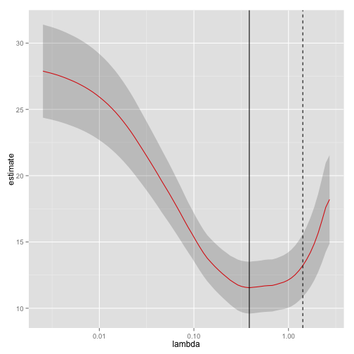
## 1 0.3853002 1.41728Why is this useful? Because we can plot it using ggplot2!
library(ggplot2)

ggplot(tidied_cv, aes(lambda, estimate)) + geom_line(color = "red") +
    geom_ribbon(aes(ymin = conf.low, ymax = conf.high), alpha = .2) +
    scale_x_log10() +
    geom_vline(xintercept = glance_cv$lambda.min) +
    geom_vline(xintercept = glance_cv$lambda.1se, lty = 2)