Since I joined Stack Exchange as a Data Scientist in June, one of my first projects has been reconsidering the A/B testing system used to evaluate new features and changes to the site. Our current approach relies on computing a p-value to measure our confidence in a new feature.
Unfortunately, this leads to a common pitfall in performing A/B testing, which is the habit of looking at a test while it’s running, then stopping the test as soon as the p-value reaches a particular threshold- say, .05. This seems reasonable, but in doing so, you’re making the p-value no longer trustworthy, and making it substantially more likely you’ll implement features that offer no improvement. How Not To Run an A/B Test gives a good explanation of this problem.
One solution is to pre-commit to running your experiment for a particular amount of time, never stopping early or extending it farther. But this is impractical in a business setting, where you might want to stop a test early once you see a positive change, or keep a not-yet-significant test running longer than you’d planned. (For more on this, see A/B Testing Rigorously (without losing your job)).
An often-proposed alternative is to rely on a Bayesian procedure rather than frequentist hypothesis testing. It is often claimed that Bayesian methods, unlike frequentist tests, are immune to this problem, and allow you to peek at your test while it’s running and stop once you’ve collected enough evidence. For instance, the author of “How Not To Run an AB Test” followed up with A Formula for Bayesian A/B Testing:
Bayesian statistics are useful in experimental contexts because you can stop a test whenever you please and the results will still be valid. (In other words, it is immune to the “peeking” problem described in my previous article).
Similarly, Chris Stucchio writes in Easy Evaluation of Decision Rules in Bayesian A/B Testing:
This A/B testing procedure has two main advantages over the standard Students T-Test. The first is that unlike the Student T-Test, you can stop the test early if there is a clear winner or run it for longer if you need more samples.
Swrve offers a similar justification in Why Use a Bayesian Approach to A/B Testing:
As we observe results during the test, we update our model to determine a new model (a posteriori distribution) which captures our belief about the population based on the data we’ve observed so far. At any point in time we can use this model to determine if our observations support a winning conclusion, or if there still is not enough evidence to make a call.
We were interested in switching to this method, but we wanted to examine this advantage more closely, and thus ran some simulations and analyses. You can find the knitr code for this analysis here, along with a package of related functions here.
We’ve concluded that this advantage of Bayesian methods is overstated, or at least oversimplified. Bayesian A/B testing is not “immune” to peeking and early-stopping. Just like frequentist methods, peeking makes it more likely you’ll falsely stop a test. The Bayesian approach is, rather, more careful than the frequentist approach about what promises it makes.
Review: the problem with using p-values as a stopping condition
The aforementioned post provides an explanation of the problem with stopping an experiment early based on your p-value, but we’ll briefly explore our own illustrative example. We currently use a simple, but common, approach, familiar to many A/B testers: a Chi-squared two-sample proportion test. Our data might look something like this:
| Clicks | Impressions | |
|---|---|---|
| A | 127 | 5734 |
| B | 174 | 5851 |
We would perform a significance test on this data and get a p-value of 0.012103, suggesting that new feature improved clickthrough rate, and we should change from A to B.
Suppose we are running an A/B test on a new feature. We run the experiment for 20 days, and on each day get about 10,000 impressions. We use the Chi-squared test for the difference between two proportions to test whether the new feature improved click-through rate. Unbeknownst to us, the new feature has absolutely no effect- the clickthrough rate is always .1%.
If we look at the results on the 20th day, we find that 5.34% of our simulations fell below our p-value cutoff of .05. The rate at which we falsely call nulls significant is called the type I error rate. By setting a p-value threshold of .05, we set a goal that that error rate should be 5%, and we (roughly) kept that promise. The system worked!
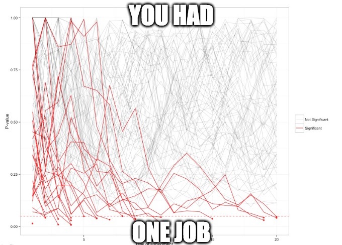
But! Suppose you recorded your p-values at the end of each day. Among a hundred experiments, you might see something like this:
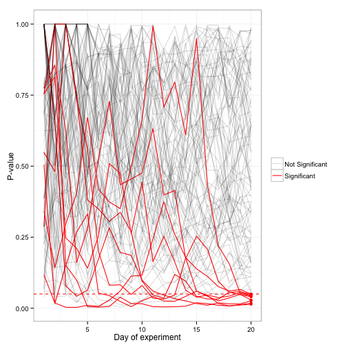
Notice that over time, each experiment’s p-value squiggled up and down before ending where it did at day 20. There are still only 5 experiments that ended with a p-value below .05 (highlighted in red). But notice that the experiment often “dips into significance” before coming back out. What if we were impatient, and stopped those experiment right then?
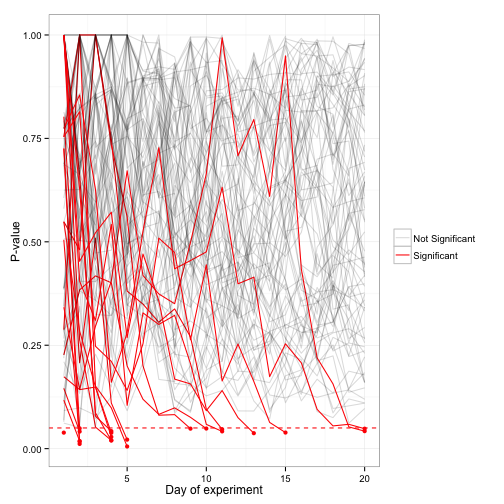
Even though none of the simulations had a real effect, 22.68% of them drop below the significance cutoff of .05 at some point. If we stopped the experiment right then, we would end up calling them significant- and our Type I error rate goes way up. Our method didn’t keep its promise!
Setting a Bayesian decision rule doesn’t avoid the peeking problem
We now consider the Bayesian decision rule proposed and examined by Evan Miller and Chris Stucchio in the posts quoted above. Like most Bayesian methods, this procedure is much less concerned with the null hypothesis than p-value testing is (indeed, it makes no promises at all about the rate at which nulls are called significant). Rather, it is concerned with the posterior expected loss: the average amount we would lose by switching from A to B.
“Expected loss” is a bit of a counterintuitive concept for those new to Bayesian methods, so it’s worth explaining more thoroughly. (Part of the confusion is that statisticians use “expected” to mean “average”- very different than how it’s used in everyday conversation). The expected loss is a combination of how probable it is that B has a lower clickthrough rate than A (the risk that you’re wrong to switch), and, if B is worse, how much worse it is on average (the potential downside). For example:
- If there is a 10% chance that B is worse, and if it is worse it decreases clickthrough rate by .0001 (a hundredth of a percent) on average, the expected loss is \(10\% \cdot .0001 = 10^{-5}\)
- If there is a 1% chance that B is worse, and if it is worse it decreases clickthrough rate by .0001 (a hundredth of a percent) on average, the expected loss is \(10\% \cdot .00001 = 10^{-6}\)
- If there is a 10% chance that B is worse, and if it is worse it decreases clickthrough rate by .00001 (a thousandth of a percent) on average, the expected loss is \(10\% \cdot .00001 = 10^{-6}\)
Notice the balance between how likely it is that you’re making a mistake in switching to B, and how much you’re giving up if you are. Also notice that we’re entirely ignoring the potential upside- the rule isn’t considering how much better A could be. As a result, the expected loss is always negative. We could choose a different rule that rewards us based on how much better A might be; we simply chose not to.
Suppose we are testing a new feature, one that (unbeknownst to us) would actually decrease our clickthrough rate from .1% to .09%. we set a “threshold of caring” of .00001, and then stop our experiment whether the expected loss falls below that threshold. Here we use a prior of \(\alpha=10;\beta=90\) (more on the choice of prior later). We run our experiment until day 20, and then make our decision.
Much like we did with the p-values, we graph the expected loss over-time of 100 of the simulations we ran:
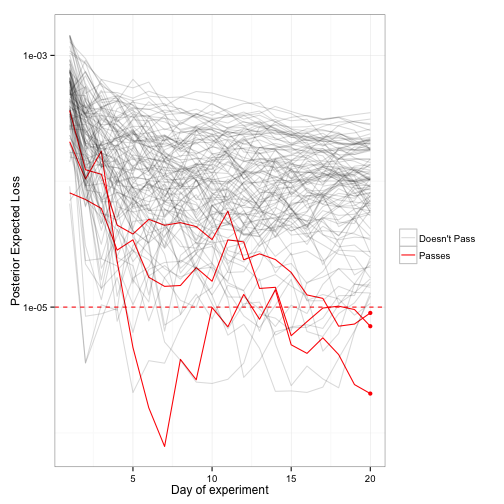
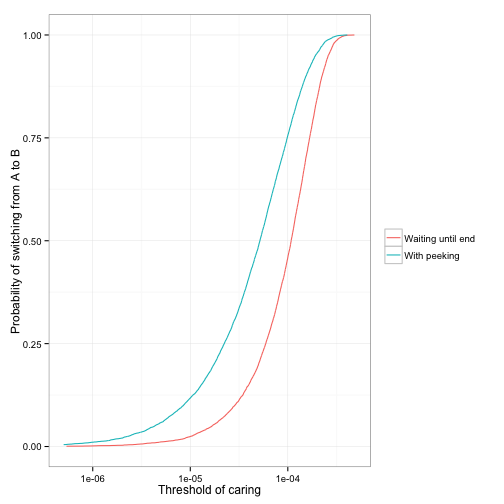
Across all our simulations, we found that the Bayesian procedure decided to change from A to B in 2.5% of cases, which seems like an acceptable risk.
What if we peeked every day, though, and were willing to stop the experiment early?
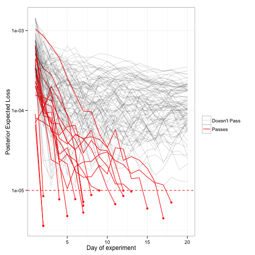
By peeking, we ended up changing from A to B in 11.8% of cases. By peeking, we made it more than four times as likely we’ll implement this change (and therefore negatively impact our clickthrough rate). This problem exists whatever threshold of caring we set:
What’s going on?
Why isn’t the Bayesian method keeping its promise of being immune to stopping? Did we make an error in our implementation of the method? Are others mistaken in their claims? No, it’s just that the Bayesian method never made this specific promise.
- Bayesian methods don’t claim to control type I error rate. It instead set a goal about the expected loss. (Side-note Due to a property called the universal bound, certain Bayesian methods have good guarantees about the error rate in the presence of stopping- but as Sanborn and Hills 2013 shows, these assumptions don’t hold for experiments, such as A/B testing, that include a composite hypothesis). In a sense, this means we haven’t solved the problem of peeking described in How Not To Run an A/B Test, we’ve just decided to stop keeping score!
- Bayesian reasoning depends on your priors being appropriate. In these simulations, we assumed that feature B was always .0001 worse than feature A, even though our prior allowed either to be better than the other. In other words, we were testing the performance on a sub-problem- how the Bayesian approach recognizes cases where a change would make things worse- but using a prior meant to work over a variety of situations.
It’s worth examining what promise the Bayesian method actually is keeping. To do that, we set up a new simulation, one where our priors are appropriate and where we can evaluate the properties directly. In each simulation, we generate the clickthrough rates of conditions A and B, separately and independently, from the same \(\beta(\alpha,\beta)\) distribution, where \(\alpha=100\) and \(\beta=99900\). The result is that in our simulation, A is better half the time, B is better half the time- sometimes by a little, sometimes by a lot. Here’s what that prior looks like:
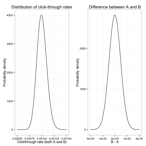
Suppose we then use those exact \(\alpha\) and \(\beta\) as our prior. That is- we have set up a perfect prior, one that exactly reflects the underlying distributions before we have any evidence.
Recall that the Bayesian method sets a “threshold of caring:” a maximum expected loss that we’re willing to accept. (Recall also that expected loss is always greater than zero- it is concerned with the sliver of a chance B is worse than A, however small that chance is). In our simulation, we can see what loss we actually end up with (that is, how often, and how much, worse B is than A on average) when we choose a threshold of caring. And we can do so either with or without optional stopping:
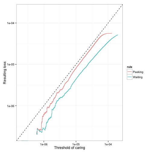
The Bayesian procedure promises to stay below the dashed line, and it does, even with the option of ending your test early. If you set a threshold of caring of \(10^{-6}\), then you might end up with a \(10\%\) chance of decreasing your click-through rate by \(.00001\), or a \(1\%\) chance of decreasing your click-through rate by \(.0001\), but not more. Notice that optional stopping brings you closer to breaking your promise (and not by a trivial amount; note that it’s a logarithmic scale). That’s OK: you’re using up the “slack” that the method gave you, in exchange for getting to stop your test as soon as you’re sure, rather than waiting the full 20 days to gather extra evidence.
But in the same process, you’re increasing your Type I error rate, the fraction of features that decrease your click-through rate but are still accepted.\({}^{[1]}\) That’s what we saw earlier in our glimpse of 100 simulations, and it’s what we see here:
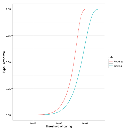
By how much are you increasing your Type I error rate? Your experimental setup doesn’t promise anything: you’ll need simulations like the ones above, or a separate Bayesian analysis, to tell you.
Note again that all this happens even when the method is provided with the best possible prior- one that actually represents the distribution of A and B clickthrough rates that are fed to it. It would be worth doing simulations where the prior is wrong: too restrictive around the predictive click-through rate, or not restrictive (informative) enough. Some preliminary results (not shown) suggest that when the prior is less representative of the distribution, the peeking problem becomes substantially more dramatic.
Which is worse: breaking a promise, or not making it at all?
Part of the reason we feel betrayed by the flaw in the frequentist approach is that p-values are already making just one promise: to control our Type I error rate. They’re sort of terrible at almost everything else. If they can’t even control our Type I error rate, then what are they good for?
In that sense, Bayesian methods are appealing: they set a goal and hold to it no matter how much you peek. Indeed, perhaps the goal they set is better: Bayesian statisticians often argue that the frequentist focus on the Type I error rate is misguided. Certainly the expected loss has a relevant business interpretation (“don’t risk decreasing our clickthrough rate”).
But maybe we should care about the error rate. A Bayesian might argue that if there’s no difference between features A and B, then there’s no cost to switching. But developers don’t make these decisions in a vacuum: a positive test could lead one to spend development time heading down the same, misguided path. (“I’ve implemented five features, each of which took a week, that all succeeded in A/B tests. But our clickthrough rate still hasn’t gone up!”) Changing approaches would require more than a modification of some software- it would require a shift in our entire mindset towards testing.
We’re not the only ones considering this phenomenon. Many researchers (some cited below) examine “frequentist properties” as part of an evaluation of Bayesian methods.
TL;DR: Why we’re not changing (yet)
At Stack Exchange, we aren’t switching to this method of Bayesian A/B testing just yet. The reasons:
- The claim of “Bayesian testing is unaffected by early stopping” is simply too strong. Stopping a Bayesian test early makes it more likely you’ll accept a null or negative result, just like in frequentist testing. And being overconfident in a statistical method is often a much greater danger than any flaws in the method itself.
- As discussed above, we’re concerned about the effect of focusing on the expected loss, and thereby letting features that offer no improvement pass the test.
- There are cognitive and cultural costs associated with changing methods. P-values can be counter-intuitive, yes. But switching to Bayesian testing requires getting everyone familiar with priors, posteriors, and the loss function- it’s trading one set of challenging concepts for another. And managing the problems discussed in this post requires even more advanced techniques: sensitivity analysis, model checking, and so on. P-values are, if nothing else, the devil we know.
- We’re concerned about the choice of priors. Choosing a more informative prior mitigates (though it doesn’t eliminate) the effect of a stopping rule, but also comes with risk to your power and robustness if your guess is wrong. A/B testing is used by several departments for many purposes, each of which would need its own priors if they are to be useful. It’s not an insurmountable obstacle, but it is an obstacle.\({}^{[2]}\)
The problem isn’t solved, so we’re looking into a few other remedies:
- Frequentist approaches to sequential testing. For example, this and this. This does have the advantage of providing a similar interface to the A/B tester, just one with an appropriately corrected p-value.
- Alternative Bayesian procedures. For example, focusing just on the expected loss may lead us to call null results significant. But if we base our procedure not just on the expected loss, but also the posterior probability \(Pr(B > A)\), we can focus on cases where we’re confident in a positive change.
- Encouraging pre-committal, and statistics familiarity Sometimes it actually is plausible to commit to running a test for a particular amount of time; and with the right power-analysis tools, we can estimate an appropriate length in advance. And to some extent, simply appreciating what a p-value means, and how the problem of optional stopping arises, can help mitigate the problem.
Conclusion
This is certainly not a blanket criticism of an entire philosophy. Some Bayesian approaches are immune to problems from optional stopping. Some frequentist approaches are as well. And there may be many other reasons you may prefer Bayesian methods. This is certainly not meant as a criticism of the authors we quote above, who were very helpful in introducing us to Bayesian A/B testing approaches.
Rather, this is an expression of caution. It may turn out that Bayesian A/B testing methods have better properties for our needs, or yours. But this should be explored through careful simulations, with a focus on the specific use case. The assumption that peeking is simply “free” in Bayesian methods can be dangerous.
We would like nothing more than to be convinced! The right mix of theory, simulations, and business considerations could certainly show that Bayesian tests are a more robust and reliable way to increase our click-through rate. But we’re not yet there. And if we do decide to change, we’ll be sure to share why.
Further Reading
Just as this is not the end of the conversation, it is not the beginning. Some relevant posts were quoted earlier, but we’ll collect them in one place:
- How Not to Run An A/B Test, by Evan Miller
- Agile A/B testing with Bayesian Statistics and Python, by Chris Stucchio (the Bayesian Witch site appears to be down, so this links to an Internet Archive version)
- A Formula for Bayesian A/B Testing, by Evan Miller
- Easy Evaluation of Decision Rules in Bayesian A/B testing, by Chris Stucchio
Other posts of interest include:
- A/B Testing Rigorously (without losing your job) and A/B Testing With Limited Data, by Ben Tilly, offer frequentist approaches to the optional stopping problem.
- Rapid A/B Testing with Sequential Analysis, by Audun M. Øygard describes another frequentist approach, the Sequential Generalized Likelihood Ratio Test.
- Optional stopping in data collection: p values, Bayes factors, credible intervals precision, by John K. Kruschke, compares several frequentist and Bayesian rules for stopping, and endorses a Bayesian rule based on waiting for a particular precision.
- Stopping rules and Bayesian analysis, by Andrew Gelman, supports the Bayesian approach to stopping. He admits that “you do lose some robustness but… robustness isn’t the only important thing out there,” and emphasizes that the problem is not so much the Bayesian procedure so much as that people are “mixing Bayesian inference with non-Bayesian decision making.”
- On the scalability of statistical procedures: why the p-value bashers just don’t get it, by Jeff Leek, doesn’t address optional stopping, but does express some deeply relevant arguments about p-values and their alternatives.
A number of scientific articles have explored this question as well, coming down on both sides of the issue. Note that some are more technical than others, and that some are behind paywalls.
- When decision heuristics and science collide. Yu, E. C., Sprenger, A. M., Thomas, R. P., & Dougherty, M. R. (2013). Psychonomic Bulletin & Review, 21(2), 268–282. http://doi.org/10.3758/s13423-013-0495-z
- Persistent Experimenters, Stopping Rules, and Statistical Inference. Steele, K. (2013). Erkenntnis, 78(4), 937–961. http://doi.org/10.1007/s10670-012-9388-1
- The frequentist implications of optional stopping on Bayesian hypothesis tests. Sanborn, A. N., & Hills, T. T. (2014). Psychonomic Bulletin & Review, 21(2), 283–300. http://doi.org/10.3758/s13423-013-0518-9
- Optional stopping: No problem for Bayesians. Rouder, J. N. (2014). Psychonomic Bulletin & Review, 21(2), 301–308. http://doi.org/10.3758/s13423-014-0595-4
- Reply to Rouder (2014): Good frequentist properties raise confidence. Sanborn, A. N., Hills, T. T., Dougherty, M. R., Thomas, R. P., Yu, E. C., & Sprenger, A. M. (2014). Psychonomic Bulletin & Review, 21(2), 309–311. http://doi.org/10.3758/s13423-014-0607-4
Footnotes
[1] In Bayesian terminology, we’re actually talking about a particular kind of Type S error- mistaking the sign of an effect. But it’s getting at the same idea: the probability that a feature that makes things worse will “slip through”.
[2] I also have concerns about treating the priors for A and B as independent Betas. Surely much of our uncertainty about the clickthrough rate affects both A and B equally- for instance, we might find it plausible the clickthrough rate for A is \(.1\%\) and for B is \(.11\%\), or that A is \(.2\%\) and B is \(.21\%\), but think it unlikely that A is \(.1\%\) and B is \(.21\%\). But I’ll save that consideration for a future post and analysis.
