
Previously in this series
- The “lost boarding pass” puzzle
- The “deadly board game” puzzle
- The “knight on an infinite chessboard” puzzle
- The “largest stock profit or loss” puzzle
- The “birthday paradox” puzzle
- The “Spelling Bee honeycomb” puzzle
- Feller’s “coin-tossing” puzzle
- The “spam comments” puzzle
I love 538’s Riddler column, and I’ve enjoyed solving the May 1st puzzle. I’ll quote:
You are locked in the dungeon of a faraway castle with three fellow prisoners (i.e., there are four prisoners in total), each in a separate cell with no means of communication. But it just so happens that all of you are logicians (of course)….
Each prisoner will be given a fair coin, which can either be fairly flipped one time or returned to the guards without being flipped. If all flipped coins come up heads, you will all be set free! But if any of the flipped coins comes up tails, or if no one chooses to flip a coin, you will all be doomed to spend the rest of your lives in the castle’s dungeon.
The only tools you and your fellow prisoners have to aid you are random number generators, which will give each prisoner a random number, uniformly and independently chosen between zero and one.
What are your chances of being released?
I’ll solve this with tidy simulation in R, in particular using one of my favorite functions, tidyr’s crossing(). In an appendix, I’ll show how to get a closed form solution for \(N=4\).
I’ve also posted a 30-minute screencast of how I first approached the simulation and visualization.
Simulating four prisoners
Before we jump into our simulation, we can start with a bit of logic. The four prisoners can’t communicate and they’re in symmetrical situations. This means we’ll all have to take the same strategy, trusting in the fact that all the other logicians will choose the same one.
If we all decided not to flip a coin, we’d never get free. If we all decided to flip the coin, our chance of freedom would be \(\frac{1}{2^4}=\frac{1}{16}\), the chance of four heads. Thus, we have one knob with which to control our strategy: the probability that we decide to flip our coin instead of returning it to the guards.
Since this probability will the be the same across all four prisoners, we can simulate this for many possible strategies between 1% and 100% using rbinom().
library(tidyverse)
library(scales)
theme_set(theme_light())
set.seed(2020-05-04)

sim <- crossing(trial = 1:100000,
                probability = seq(.01, 1, .01)) %>%
  mutate(num_flips = rbinom(n(), 4, probability),
         num_tails = rbinom(n(), num_flips, .5),
         set_free = num_flips != 0 & num_tails == 0)

sim
## # A tibble: 10,000,000 x 5
## trial probability num_flips num_tails set_free
## <int> <dbl> <int> <int> <lgl>
## 1 1 0.01 0 0 FALSE
## 2 1 0.02 0 0 FALSE
## 3 1 0.03 0 0 FALSE
## 4 1 0.04 0 0 FALSE
## 5 1 0.05 0 0 FALSE
## 6 1 0.06 1 0 TRUE
## 7 1 0.0700 0 0 FALSE
## 8 1 0.08 0 0 FALSE
## 9 1 0.09 1 0 TRUE
## 10 1 0.10 0 0 FALSE
## # … with 9,999,990 more rowsThe above performs 10 million simulations (100,000 trials for each probability) but because it’s vectorized it’s pretty fast: about 1.5 seconds on my machine. Notice that the prisoners are set free only if they flip at least one coin and get no tails (num_flips != 0 & num_tails == 0). In the first ten simulations above, the strategy appeared to work twice (the 6th and 9th observations).
Each value of probability is one strategy: the probability each prisoner decides to use to see if they’ll flip their coin. We can thus summarize and visualize the chance of freedom within each probability.
summarized <- sim %>%
  group_by(probability) %>%
  summarize(pct_free = mean(set_free))

summarized %>%
  ggplot(aes(probability, pct_free)) +
  geom_line() +
  expand_limits(y = 0)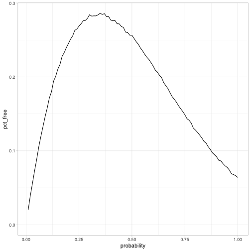
This curve makes some intuitive sense. If the probability of flipping is too low, there’s a high risk that nobody flips a coin, but if the probability is too high it approaches \(\frac{1}{16}\). We also knew the peak couldn’t be above 50%, since at least one coin will have to get flipped.
summarized %>%
  arrange(desc(pct_free))
## # A tibble: 100 x 2
## probability pct_free
## <dbl> <dbl>
## 1 0.35 0.286
## 2 0.37 0.286
## 3 0.36 0.285
## 4 0.3 0.284
## 5 0.34 0.284
## 6 0.32 0.283
## 7 0.33 0.283
## 8 0.31 0.282
## 9 0.38 0.282
## 10 0.39 0.282
## # … with 90 more rowsIt looks like the optimum is around 35% (though there’s some uncertainty), and that when they use that strategy the prisoners will have a 28% chance of release.
Exact solution with optimize
To move from a simulation to an exact solution, let’s start by getting the exact formula for that curve. What’s the probability the prisoners go free if the chance of each flipping their coin is p?
There are four ways that we wind up winning: 1 prisoner can flip 1 heads, 2 prisoners can flip 2 heads, 3 prisoners can flip 3 heads, and 4 prisoners could flip 4 heads. These are disjoint events (it’s impossible two of them happen together), so we can sum up the probabilities. Let F be the number of coins that are flipped, and T be the number of tails flipped. The probability of getting freedom is
\[\sum_{k=1}^4{P(F=k|p)P(T=0|F=k)}\]Both of these probabilities follow a binomial distribution: the probability of some number of successes in a set of idential trials. And the probability there are no tails is \(\frac{1}{2^k}\) This can be written in R as follows, using the dbinom() function:
probability_exact <- function(p, n = 4) {
  sum(dbinom(1:n, n, p) / 2 ^ (1:n))
}

# Probability all heads if each player has 20% chance
probability_exact(.2)
## [1] 0.2465We could add these exact values onto our earlier simulation to check our math.
# map_dbl lets us calculate probability of freedom for each strategy
summarized %>%
  mutate(exact = map_dbl(probability, probability_exact)) %>%
  ggplot(aes(probability, pct_free)) +
  geom_line() +
  geom_line(aes(y = exact), color = "red", lty = 2) +
  expand_limits(y = 0)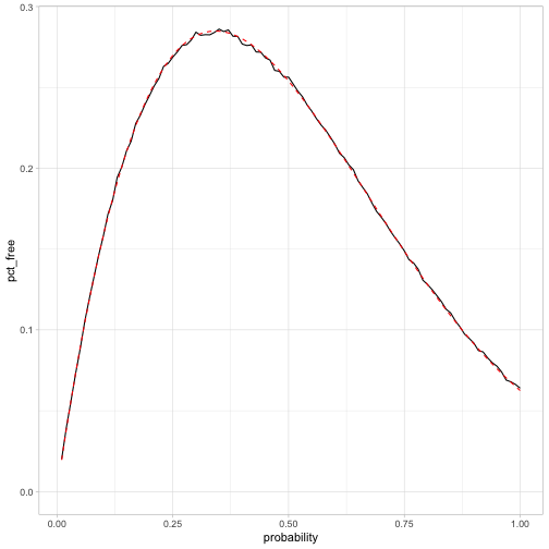
This matches the simulation, so it looks like we got it right!
We’re especially interested in the peak: what’s the optimal strategy, and the corresponding probability of going free? We can use the built-in optimize function, which is built for one-dimensional optimization within an interval.
opt <- optimize(probability_exact, c(0, 1), maximum = TRUE)
opt
## $maximum
## [1] 0.3420391
##
## $objective
## [1] 0.2848424The highest chance of escape is 28.5%, when the prisoners use the random number generator to have a 34.2% chance of flipping the coin.
If you want to see some equations rather than simulations, the Appendix below shows how to calculate the (slightly messy) exact form, and gets some hints about what it looks like for an arbitrary N.
Extra credit: arbitrary N
Extra credit: Instead of four prisoners, suppose there are N prisoners. Now what are your chances of being released?
What’s wonderful about the crossing() function is that we can always add another variable to our calculation. Let’s add n, ranging from 2 prisoners to 8 prisoners.
sim_n <- crossing(trial = 1:100000,
                  probability = seq(.02, 1, .02),
                  n = 2:8) %>%
  mutate(num_flips = rbinom(n(), n, probability),
         num_tails = rbinom(n(), num_flips, .5),
         set_free = num_flips != 0 & num_tails == 0)
Since our probability_exact() function takes two arguments (p and n), we can also calculate all the exact probabilities with map2_dbl.
probabilities_n <- sim_n %>%
  group_by(probability, n) %>%
  summarize(simulated = mean(set_free)) %>%
  ungroup() %>%
  mutate(exact = map2_dbl(probability, n, probability_exact))

probabilities_n %>%
  ggplot(aes(probability, exact, color = factor(n))) +
  geom_line() +
  geom_point(aes(y = simulated), size = .4) +
  scale_x_continuous(labels = percent) +
  scale_y_continuous(labels = percent) +
  labs(x = "p: Probability of flipping the coin",
       y = "Probability of freedom",
       color = "N: # of prisoners",
       title = "What's the chance of escaping with n prisoners?",
       subtitle = "Points show simulations of 100,000 prisoners each; lines are exact solution")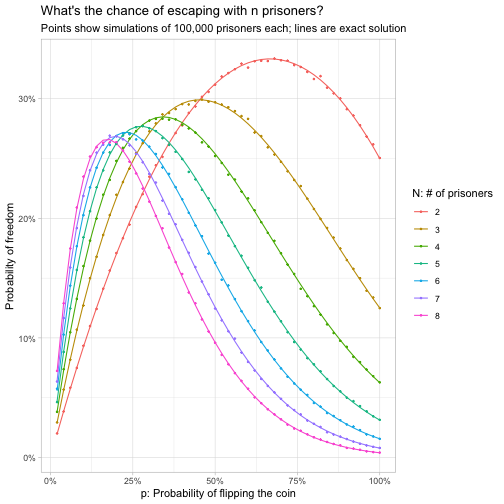
This let us check our results for an arbitrary $N$. It looks like our simulation and exact calculations line up, which is a good way to check our work!
The probability of freedom has one peak for any value of $N$. It looks like the best value of \(p\) when there are two prisoners is about a 2/3 chance of flipping, and that decreases as \(N\) increases. The chance of success also decreases as \(N\) increases, but not by too much, and it looks like it might asymptote.
Let’s use optimize to find the best strategy for every value of \(N\), up to (say) 60 prisoners.
# Function that takes n and runs the optimise step
optimize_for_n <- function(n) {
  optimize(function(p) probability_exact(p, n), c(0, 1), maximum = TRUE)
}

optimal_n <- tibble(n = 2:60) %>%
  mutate(optimal = map(n, optimize_for_n)) %>%
  unnest_wider(optimal)

optimal_n %>%
  gather(metric, value, -n) %>%
  mutate(metric = ifelse(metric == "maximum", "Optimal probability to flip", "Probability of escape")) %>%
  ggplot(aes(n, value, color = metric)) +
  geom_line() +
  geom_hline(lty = 2, yintercept = .25) +
  scale_y_continuous(labels = percent) +
  expand_limits(y = 0) +
  labs(x = "N: # of prisoners",
       y = "Probability",
       color = "",
       title = "How does the optimal strategy and outcome change with N?")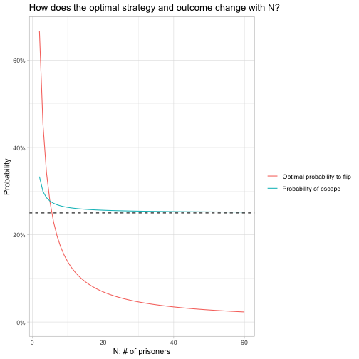
The optimal \(p\) does indeed decrease as \(N\) increases, and appears to be approaching zero. The probability of escape (you’d rather play this game with just one other prisoner than with many), but notice that it is approaching an asymptote, which appears to be 25% (shown as a dashed line).
Instead of thinking about the optimal value of \(p\), it might make sense to think about \(Np\), the expected number of flips. That is, how many flips are you aiming for across all \(N\) prisoners?
optimal_n %>%
  arrange(desc(n)) %>%
  mutate(expected_coins_flipped = n * maximum) %>%
  ggplot(aes(n, expected_coins_flipped)) +
  geom_line() +
  labs(y = "Expected # of coins getting flipped")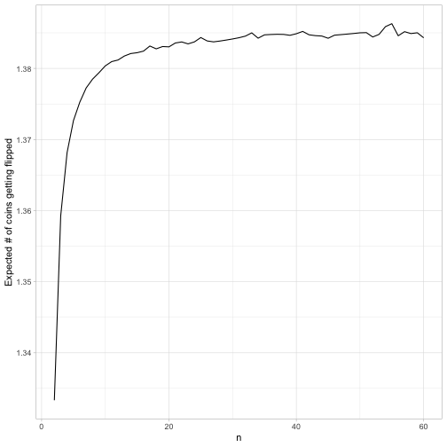
With a small \(N\) you’re looking to flip about 1.34 coins, and as \(N\) gets large that target seems to approach 1.386.
It makes intuitive sense that you’re aiming at a number of flips a little over 1. You really don’t want to end up flipping zero (in which case you’ll lose right away), but you’re balancing that against not wanting to flip too many, in which case you’ll have a high risk of flipping at least one tails.
As \(N\) gets large, since \(p\) stays small, the number of coins flipped will approach a Poisson distribution, a useful distribution of counts where the variance is equal to the mean. At that point, it doesn’t end up mattering what \(N\) is, so it makes sense that the probability of escape asymptotes rather than continuing to decline.
# Summing the Poisson probabilities up to 1000
optimize(function(p) sum(dpois(1:1000, p) / 2 ^ (1:1000)),
         c(0, 10),
         maximum = TRUE)
## $maximum
## [1] 1.386312
##
## $objective
## [1] 0.25Put another way: even if you were playing this game with a billion prisoners, you’d still have a 25% chance of escaping: each prisoner would just take a \(\frac{1.386}{1,000,000,000}\) chance of flipping the coin. Pretty cool!
(I don’t have an intuition for why the optimal expected number of flips is 1.386, or why the probability of escape approaches \(\frac{1}{4}\), but I bet someone who’s good with infinite series could work it out based on the density of the Poisson distribution).
Appendix: Closed form solution for N=4
I focus more on code than on equations in this blog, but I thought I’d try getting an exact form for the optimal strategy. After all, I’d have to if I were one of the prisoners and didn’t have access to R.
\[\sum_{k=1}^4{P(F=k|p)P(T=0|F=k)}\] \[=\sum_{k=1}^4\frac{ {4 \choose k} p^k(1-p)^{4-k}}{2^k}\] \[=\frac{4p(1-p)^3}{2}+\frac{6p^2(1-p)^2}{4}+\frac{4p^3(1-p)}{8}+\frac{p^4}{16}\] \[=2p(1-p)^3+\frac{3}{2}p^2(1-p)^2+\frac{1}{2}p^3(1-p)+\frac{1}{16}p^4\] \[=2p(1-p)^3+\frac{3}{2}p^2(1-p)^2+\frac{1}{2}p^3(1-p)+\frac{1}{16}p^4\] \[=-\frac{15}{16}p^4+\frac{7}{2}p^3-\frac{9}{2}p^2+2p\]We can see from the graph above that there is one maximum between 0 and 1. To find that maximum, we’ll take the derivative and set it to zero:
\[0=-\frac{60}{16}p^3+\frac{21}{2}p^2-9p+2\]Life is too short for me to remember how to find the roots of cubic equations (though I hope for their sake that the prisoners can work it out), but Wolfram Alpha tells me the only solution is:
\[-\frac{2}{15}(-7+2^{1/3}+2 \times 2^{2/3})\]So… if you had that closed form solution on your bingo card, congrats. But it is indeed about equal to .342, so it checks out with our simulation! I never get tired of how simulation can help check our math.
I ran through the solution (not shown) for \(n=3\) and \(n=2\), and found that they are, respectively, \(\frac{1}{7}(6-2\sqrt{2})\) and \(\frac{2}{3}\). So there are some hints at structures in common (\(2^N-1\) in the denominator, a sequence of \(N-1\)th roots of 2), but it’s not something I’m planning to solve!