
Previously in this series
- The “lost boarding pass” puzzle
- The “deadly board game” puzzle
- The “knight on an infinite chessboard” puzzle
- The “largest stock profit or loss” puzzle
- The “birthday paradox” puzzle
- The “Spelling Bee honeycomb” puzzle
- Feller’s “coin-tossing” puzzle
- The “spam comments” puzzle
- The “prisoner coin flipping” puzzle
I love 538’s Riddler column, and I’ve enjoyed solving the November 20th puzzle. I’ll quote:
To celebrate Thanksgiving, you and 19 of your family members are seated at a circular table (socially distanced, of course). Everyone at the table would like a helping of cranberry sauce, which happens to be in front of you at the moment.
Instead of passing the sauce around in a circle, you pass it randomly to the person seated directly to your left or to your right. They then do the same, passing it randomly either to the person to their left or right. This continues until everyone has, at some point, received the cranberry sauce.
Of the 20 people in the circle, who has the greatest chance of being the last to receive the cranberry sauce?
I’ll solve this with tidy simulation in R, as usual using one of my favorite functions, tidyr’s crossing(), and getting another chance to explore a variation of a “random walk”.
Simulating a table of 20
What’s fun about this problem is that it’s an example of a random walk: a stochastic process made up of a sequence of random steps (in this case, left or right). What makes this a fun variation is that it’s a random walk in a circle- passing 5 to the left is the same as passing 15 to the right. I wasn’t previously familiar with a random walk in a circle, so I approached it through simulation to learn about its properties.
Simulating a random walk in a circle
The classic way to simulate a random walk in R is with cumsum() and sample(). sample(c(1, -1)) picks a random direction for each step, and cumsum() takes the cumulative sum of those steps:
cumsum(sample(c(1, -1), 30, replace = TRUE))## [1] 1 2 3 4 5 6 7 6 5 6 5 6 5 6 7 6 5 6 7 6 5 6 5 4 5 4 3 4 5 4Right now this is a random walk on integers (…, -2, -1, 0, 1, 2, …). To make this a random walk at a circular table of 20, you can use the modulo operator, %% 20.
cumsum(sample(c(1, -1), 30, replace = TRUE)) %% 20## [1] 1 0 19 18 17 16 17 18 19 18 19 18 19 18 17 18 19 0 19 0 19 0 1 2 1 2 3
## [28] 4 5 4Notice that the cranberry sauce can now be passed from 0 to 19 and then back.
Simulating many walks with crossing()
We’ll simulate 50,000 trials (feel free to increase or decrease that number, depending on how accurate you need your simulation to be). For each, we’ll try 1000 steps.
library(tidyverse)

# For the sake of efficiency, perform only the cumulative sum
# as a grouped operation
sim_steps <- crossing(trial = 1:50000,
                      step = 1:1000) %>%
  mutate(direction = sample(c(1, -1), n(), replace = TRUE)) %>%
  group_by(trial) %>%
  mutate(position = cumsum(direction)) %>%
  ungroup() %>%
  mutate(seat = position %% 20)

sim_steps
## # A tibble: 50,000,000 x 5
## trial step direction position seat
## <int> <int> <dbl> <dbl> <dbl>
## 1 1 1 1 1 1
## 2 1 2 -1 0 0
## 3 1 3 -1 -1 19
## 4 1 4 1 0 0
## 5 1 5 -1 -1 19
## 6 1 6 1 0 0
## 7 1 7 -1 -1 19
## 8 1 8 1 0 0
## 9 1 9 1 1 1
## 10 1 10 1 2 2
## # … with 49,999,990 more rowsWe end up with 10 million steps, each representing the position of the cranberry sauce at one point in time.
How long does it take for the cranberry sauce to reach each seat for the first time? We can use distinct() with .keep_all = TRUE to answer that: we keep the first time each seat appears in each trial. (We also filter out seat 0, which is you, because you start with the cranberry sauce on step 0).
sim <- sim_steps %>%
  distinct(trial, seat, .keep_all = TRUE) %>%
  filter(seat != 0)

sim
## # A tibble: 949,995 x 5
## trial step direction position seat
## <int> <int> <dbl> <dbl> <dbl>
## 1 1 1 1 1 1
## 2 1 3 -1 -1 19
## 3 1 10 1 2 2
## 4 1 14 -1 -2 18
## 5 1 43 -1 -3 17
## 6 1 50 -1 -4 16
## 7 1 63 -1 -5 15
## 8 1 64 -1 -6 14
## 9 1 65 -1 -7 13
## 10 1 66 -1 -8 12
## # … with 949,985 more rowsSummarizing and visualizing
Now that we have our simulation with one row for each seat in each trial, we can learn stats about each seat. Which is the best seat to be in? Which is most likely to be last?
by_seat <- sim %>%
  group_by(trial) %>%
  mutate(is_last = row_number() == 19) %>%
  group_by(seat) %>%
  summarize(avg_step = mean(step),
            pct_last = mean(is_last),
            avg_length_last = mean(step[is_last]))
This isn’t the Riddler’s question, but it’s the first one I was interested in: how long does it take for each seat, on average, to get the cranberry sauce?
by_seat %>%
  ggplot(aes(seat, avg_step)) +
  geom_line() +
  expand_limits(y = 0) +
  labs(x = "Seat",
       y = "Average # of steps to reach this seat")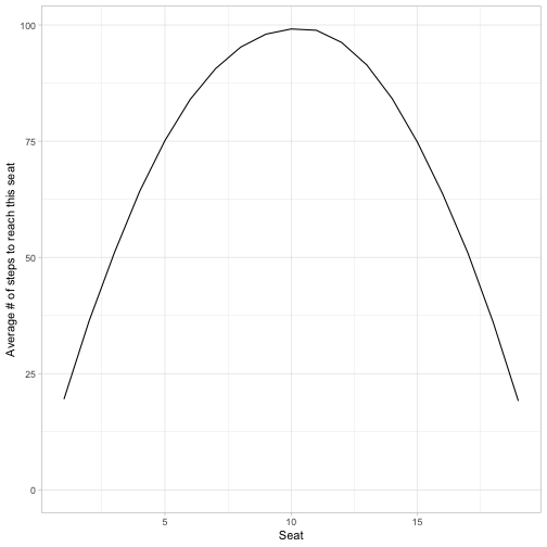
It looks like a parabola. The best seat to be in is either #1 or #19, immediately to the right or left of the starting position: on average they’re waiting about 19 steps to get it. The worst seat to be in is #10, directly across the table. On average they’re waiting about 100 steps to get it. Overall, this makes intuitive sense: the closer you are to the original sauce, the more likely you can get it right away.
What I love about tidy simulation is that I can visualize some more details about the distribution, such as with a histogram on a log scale.
sim %>%
  ggplot(aes(step)) +
  geom_histogram() +
  scale_x_log10() +
  facet_wrap(~ seat, scales = "free_y") +
  labs(x = "Step on which this seat gets the cranberry sauce",
       y = "")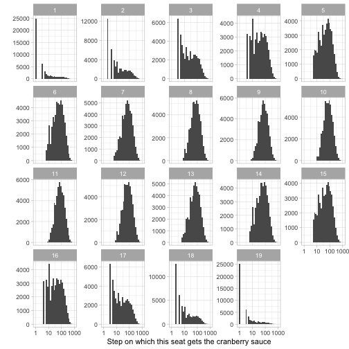
The seats immediately to your left and right, 1 and 19, have a mode of 1 step (which makes sense: they have a 50% chance of getting it on the first step). For seats that are roughly across the table (like 7-13), the number of steps looks roughly log-normally distributed.
Now let’s answer the Ridder’s question: how likely is each seat to be the last person to get the cranberry sauce?
by_seat %>%
  ggplot(aes(seat, pct_last)) +
  geom_line() +
  scale_y_continuous(labels = scales::percent) +
  geom_hline(yintercept = 1 / 19, lty = 2, color = "red") +
  expand_limits(y = 0) +
  labs(x = "Seat",
       y = "% this is the last seat to get cranberry sauce")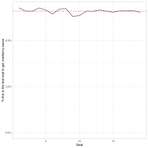
That’s a very different story! Other than a little random noise, the 19 people at the table all have the same probability of being the last to receive the cranberry sauce. (The probability is therefore 1/19, shown by the dashed red line).
This wasn’t what I originally expected, but upon consideration it makes sense. Consider the person at seat 10 (directly across the table from you). We know it will take longer for them to get the sauce, but consider what it would take to be last. Imagine the moment that the sauce first reaches either person 9 or person 11 (one of which has to happen first). At that moment, the situation is analogous. to the person seated immediately to the original left or right: the sauce would have to make a full circle of the table before going just one step. The same would apply to any seat \(s\), by breaking it down into the situation where the sauce reaches either \(s-1\) or \(s+1\).
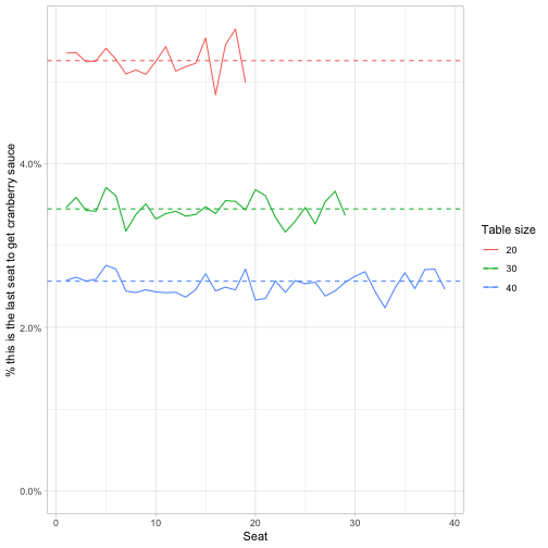
Larger table sizes
Something I love about crossing() for simulation is that you can keep adding complexity to the question you’re asking. What if there weren’t 20 people at the table, but some arbitrary \(n\)? We’ll try 20, 30, and 40, doing 20K simulations each.
# Repeat all of the above, but with an extra crossing() step
sim_size <- crossing(trial = 1:20000,
                           step = 1:2000) %>%
  mutate(direction = sample(c(1, -1), n(), replace = TRUE)) %>%
  group_by(trial) %>%
  mutate(position = cumsum(direction)) %>%
  ungroup() %>%
  crossing(table_size = c(20, 30, 40)) %>%
  mutate(seat = position %% table_size) %>%
  distinct(table_size, trial, seat, .keep_all = TRUE) %>%
  filter(seat != 0)

# Group by table_size as well
by_seat_size <- sim_size %>%
  group_by(table_size, trial) %>%
  mutate(is_last = row_number() == table_size - 1) %>%
  group_by(table_size, seat) %>%
  summarize(avg_step = mean(step),
            pct_last = mean(is_last),
            avg_length_last = mean(step[is_last]))
We can confirm that the “all seats are equally likely to get the sauce last” holds true for every table size.
But we can also take a closer look at that parabola for the average # of steps to reach each position. Can we figure out a closed form solution for it?
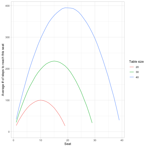
A few patterns we notice, where \(n\) is the table size.
- The peak for each is at seat \(n / 2\), which takes on average \((n / 2) ^ 2 steps\).
- The average for seats 1 and \(n-1\) (the people seated immediately to your left/right) is \(n-1\).
We can get a bit more precise by fitting a parabola to each of the seat size results, using the broom package to combine the linear models.
by_seat_size %>%
  mutate(linear = seat,
         quadratic = seat ^ 2) %>%
  group_by(table_size) %>%
  summarize(mod = list(lm(avg_step ~ quadratic + linear)),
            td = map(mod, broom::tidy, conf.int = TRUE)) %>%
  unnest(td) %>%
  ggplot(aes(table_size, estimate)) +
  geom_line() +
  geom_ribbon(aes(ymin = conf.low, ymax = conf.high), alpha = .1) +
  facet_wrap(~ term)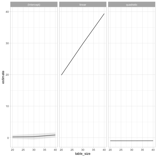
The intercept is indistinguishable from 0, the linear term is equal to the table size, and the quadratic term stays at -1. This suggests that the average number of steps to reach a seat \(s\) is \(-s^2+n*s\). (This matches our results for the maximum and the \(s=1\) point above).
As I often note in these posts, I love how doing some simulation can lead us to an exact solution (even if we can’t yet prove it).