
Last Friday’s “The Riddler” column on FiveThirtyEight presents an interesting probabilistic puzzle:
While traveling in the Kingdom of Arbitraria, you are accused of a heinous crime. Arbitraria decides who’s guilty or innocent not through a court system, but a board game. It’s played on a simple board: a track with sequential spaces numbered from 0 to 1,000. The zero space is marked “start,” and your token is placed on it. You are handed a fair six-sided die and three coins. You are allowed to place the coins on three different (nonzero) spaces. Once placed, the coins may not be moved.
After placing the three coins, you roll the die and move your token forward the appropriate number of spaces. If, after moving the token, it lands on a space with a coin on it, you are freed. If not, you roll again and continue moving forward. If your token passes all three coins without landing on one, you are executed. On which three spaces should you place the coins to maximize your chances of survival?
(There are also two variations offered, for which I present solutions afterwards).
Last year I took a look at the “lost boarding pass” puzzle in R, and I found it a useful example of using simulation to answer probabilistic puzzles. Much like the boarding pass puzzle, this has recursive relationships between each round and the previous choices, making it nontrivial to simulate. And much like the other puzzle, performing simulations can be a way to gain insight towards an exact solution.
Simpler version: one choice, 50 spaces
It’s often good to start with a simpler version of a puzzle. Here, let’s consider the case where:
- We have only 1 coin to place, not 3
- There are only 50 spaces, not 1000
Well, to sample a random roll we would use the sample function with replace = TRUE, and can turn those into positions with the cumsum() (cumulative sum) function:
set.seed(2016-10-18)
cumsum(sample(6, 20, replace = TRUE))
## [1] 4 7 10 12 13 16 18 23 29 30 35 40 45 46 52 58 59 63 66 71In this simulation the player rolled a 4, then 3, then 3, getting to positions 4, 7, and 10. It’s easy to perform this for many rolls and many trials with the replicate function. I’ll sample 50 rolls in each trial.1
set.seed(2016-10-18)
num_rolls <- 50
max_position <- 50
trials <- 200000

# create a 50 x 10 matrix of cumulative positions
# Each row is a turn and each column a trial
positions <- replicate(trials, cumsum(sample(6, num_rolls, replace = TRUE)))
positions[1:6, 1:6]
## [,1] [,2] [,3] [,4] [,5] [,6]
## [1,] 4 4 3 2 3 1
## [2,] 7 5 7 7 6 2
## [3,] 10 11 11 8 8 4
## [4,] 12 16 14 14 13 6
## [5,] 13 22 16 18 19 7
## [6,] 16 28 19 23 20 8We end up with 50 rows (one for each roll) and 10 columns (one for each trial), each containing a random simulation. For example, the first player ended up in position 4, then 7, then 10, and so on. The next went from 4 to 5 to 11.
We want to place our one coin in the most likely position, which means we just have to count the number of times each space (up to space 50) is visited. We can use the (built in) tabulate function to do so2:
count_per_position <- tabulate(positions, max_position)
count_per_position
## [1] 33078 39284 45305 52811 61869 72038 50617 53673 55955 57916 58285
## [12] 58386 55987 56850 57528 57205 57107 57036 56925 57170 57446 57326
## [23] 57316 56875 57156 57101 57167 57046 57282 57183 57592 56723 57148
## [34] 57281 56971 57088 57274 57256 57543 56971 57217 57194 57186 57159
## [45] 56807 57286 57137 57242 57189 57066I’m going to stick these results into a data frame for easy analysis later:
library(dplyr)

position_probs <- data_frame(position = seq_len(max_position),
                              probability = count_per_position / trials)

position_probs
## # A tibble: 50 × 2
## position probability
## <int> <dbl>
## 1 1 0.165390
## 2 2 0.196420
## 3 3 0.226525
## 4 4 0.264055
## 5 5 0.309345
## 6 6 0.360190
## 7 7 0.253085
## 8 8 0.268365
## 9 9 0.279775
## 10 10 0.289580
## # ... with 40 more rowsInterpreting the results
Let’s start by visualizing the probability of landing on each space. (I’m using theme_fivethirtyeight from ggthemes in honor of the source of the puzzle).
library(ggplot2)
library(ggthemes)
theme_set(theme_fivethirtyeight() +
            theme(axis.title = element_text()))

ggplot(position_probs, aes(position, probability)) +
  geom_line()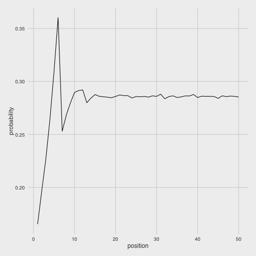
First, we notice that each position gets increasingly more likely up to 6, before diving back down. The pattern repeats itself more mildly up to 12, then basically stabilizes.
That the probabilities climb up to 6 makes sense, because there’s only a 1/6 chance of landing on 1 (you have to get it on your first roll), but there are many ways of ending up on 6 (you could roll it directly, roll 1 then 5, two 3s, three 2s, etc). The drop to 7 then makes sense because there is no longer the 1/6 possibility of landing on it on your first roll. So what would be the best spaces to pick if you had only one coin to place?
position_probs %>%
  arrange(desc(probability))
## # A tibble: 50 × 2
## position probability
## <int> <dbl>
## 1 6 0.360190
## 2 5 0.309345
## 3 12 0.291930
## 4 11 0.291425
## 5 10 0.289580
## 6 31 0.287960
## 7 39 0.287715
## 8 15 0.287640
## 9 21 0.287230
## 10 22 0.286630
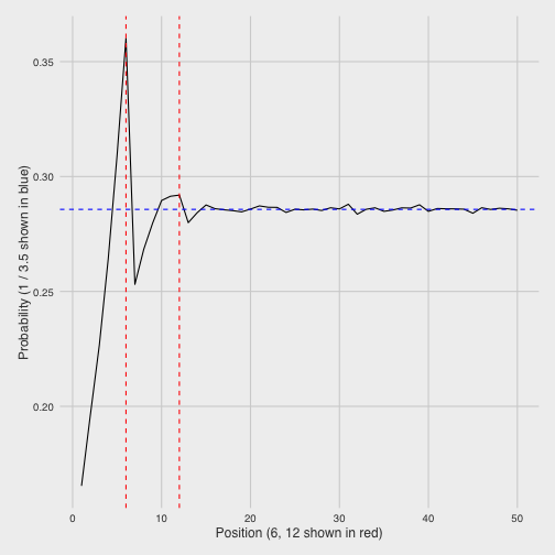
## # ... with 40 more rows6, 5, 12, 11, and 10 (the ends of those periodic cycles) were the only spaces that were better than the stabilizing probability that the later positions get stuck in.
What is that stabilizing state? Well, consider that the average roll of a six-sided die (the average of its six faces) is \((1 + 2 + 3 + 4 + 5 + 6) / 6=3.5\). This means that in the long run, we’d expect the die to move about 3.5 spaces each round- which means it would hit one out of every 3.5 spots. So if it stabilized around any one number, it would make sense for it to be 1/3.5 (2/7), which looks right:
In fact, on reflection it’s fairly straightforward to calculate the exact probabilities for each space by defining a recursive relationship between each position and the previous ones. We could notice that:
- For each position, the probability is the average of the probabilities of the previous 6 positions
- We define the position 0 to have a probability of 1 (you always start there), and negative positions to a have a probability of 0.
We can execute this simulation with a for loop or a functional approach3:
# with a for loop:
exact <- 1
for (i in seq_len(50)) {
  exact <- c(exact, sum(tail(exact, 6)) / 6)
}
exact <- exact[-1]

# alternative version with purrr::reduce
exact <- purrr::reduce(seq_len(51), ~ c(., sum(tail(., 6)) / 6))[-1]

exact
## [1] 0.1666667 0.1944444 0.2268519 0.2646605 0.3087706 0.3602323 0.2536044
## [8] 0.2680940 0.2803689 0.2892885 0.2933931 0.2908302 0.2792632 0.2835397
## [15] 0.2861139 0.2870714 0.2867019 0.2855867 0.2847128 0.2856211 0.2859680
## [22] 0.2859437 0.2857557 0.2855980 0.2855999 0.2857477 0.2857688 0.2857356
## [29] 0.2857010 0.2856918 0.2857075 0.2857254 0.2857217 0.2857138 0.2857102
## [36] 0.2857117 0.2857151 0.2857163 0.2857148 0.2857137 0.2857136 0.2857142
## [43] 0.2857146 0.2857145 0.2857142 0.2857141 0.2857142 0.2857143 0.2857143
## [50] 0.2857143We can compare this (in red) to our simulated values to confirm we got it right:
Three coins to place
We’ll now try the original version of the problem, where we place three coins. Why not just pick the three individually most likely spaces (5, 6, and 12) and call it a day? Because the probability of landing on these spaces is not independent. We need to maximize the chance we land on any space if we want to survive, and perhaps choosing 5, 6, and 12 includes “redundancies,” where we are likely.
One common necessity in simulations is to rearrange your data into. Let’s rearrange our simulated data positions into a binary matrix that I’m calling boards. Here instead of having one row for each turn, there will be one row for each space on the board. We’ll then place 1s at all the spaces where you landed. To do this, we’ll use a trick for using a two-column matrix as indices that we originally used in the boarding pass post.
# create a two-column matrix of position and trial number
position_indices <- cbind(c(positions), rep(seq_len(trials), each = num_rolls))
position_indices <- position_indices[position_indices[, 1] <= max_position, ]

# create an empty integer matrix, set those positions to 1
boards <- matrix(0L, nrow = num_rolls, ncol = trials)
boards[position_indices] <- 1L

dim(boards)
## [1] 50 200000boards[1:10, 1:6]## [,1] [,2] [,3] [,4] [,5] [,6]
## [1,] 0 0 0 0 0 1
## [2,] 0 0 0 1 0 1
## [3,] 0 0 1 0 1 0
## [4,] 1 1 0 0 0 1
## [5,] 0 1 0 0 0 0
## [6,] 0 0 0 0 1 1
## [7,] 1 0 1 1 0 1
## [8,] 0 0 0 1 1 1
## [9,] 0 0 0 0 0 1
## [10,] 1 0 0 0 0 0For example, we can see that the first simulation landed on 4, 7, and 10, and the second on positions 4 and 5.
Why construct it this way? Because it makes it easy to evaluate a three-coin strategy. For example, how well would we do if we choose spaces 1, 2, and 3? We can simply ask how many trials we landed in at least one of them:
# get first three rows of boards
mean(colSums(boards[1:3, ]) > 0)
## [1] 0.500225It looks like we’d win about half the time (which makes sense- we’d have to get a 1-3 as the first roll). What about choosing 4, 5, and 6?
mean(colSums(boards[4:6, ]) > 0)## [1] 0.79342We’d do a good deal better, with an almost 80% chance of surviving.
Let’s brute force this by trying all possible three-coin strategies between 1 and 20. (Since the per-space probability, it looks very unlikely that the best strategies will need to go past 20 spaces. A strategy of picking 5, 6 and 20 isn’t going to be that different than picking 5, 6, and 500). The combn function is useful for this, creating a matrix with one row for each of the 1140 three-coin choices:
strategies <- combn(20, 3)

dim(strategies)
## [1] 3 1140strategies[, 1:6]## [,1] [,2] [,3] [,4] [,5] [,6]
## [1,] 1 1 1 1 1 1
## [2,] 2 2 2 2 2 2
## [3,] 3 4 5 6 7 8For each of these strategies (each column in the matrix), we do the same “probability-of-winning” calculation as before.
calculate_success <- function(choice) mean(colSums(boards[choice, ]) > 0)

# use apply to perform this function on each column of strategies
probabilities <- apply(strategies, 2, calculate_success)
This is by far the slowest step of the simulation, and it gets slower still if you consider more than 20 spaces. (See the Appendix for a faster matrix-based method when working with two coins).
Which three-coin strategies maximized your probability of surviving?
# Restructure the strategies matrix into a three-column data frame
strategy_df <- as_data_frame(t(strategies))

# now add in the probabilities and sort:
best_options <- strategy_df %>%
  mutate(probability = probabilities) %>%
  arrange(desc(probability))

best_options
## # A tibble: 1,140 × 4
## V1 V2 V3 probability
## <int> <int> <int> <dbl>
## 1 4 5 6 0.793420
## 2 5 6 7 0.759905
## 3 3 5 6 0.755580
## 4 5 6 8 0.755060
## 5 5 6 9 0.744740
## 6 5 6 13 0.735625
## 7 5 6 14 0.731195
## 8 5 6 10 0.730910
## 9 5 6 15 0.728470
## 10 5 6 19 0.727695
## # ... with 1,130 more rowsWe notice that most of the top strategies include 5 and 6 in them, which were the two best choices for our “choose one” version of the game. However, the version that beat everything else (and not by a small amount) was to choose 4-5-6: and even though 4 on its own was not a particularly high probability space.
We can visualize the 25 best choices to see what else they have in common:
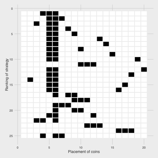
We notice that 5 and 6 dominate most strategies, and when we move away from them we tend to focus on consecutive triplets (like 10-11-12 or 9-10-11).
This makes sense in terms of interdependence among choices. Once you’re already picking 5 and 6, you should pick ones that are less likely to co-occur with those two to maximize your chances of hitting at least one. This includes ones that are immediately adjacent (4 or 7).
To review, here’s all the code we used to solve the puzzle, in one place:
set.seed(2016-10-18)
num_rolls <- 50
max_position <- 50
trials <- 200000

positions <- replicate(trials, cumsum(sample(6, num_rolls, replace = TRUE)))

position_indices <- cbind(c(positions), rep(seq_len(trials), each = num_rolls))
position_indices <- position_indices[position_indices[, 1] <= max_position, ]

boards <- matrix(0L, nrow = num_rolls, ncol = trials)
boards[position_indices] <- 1L

calculate_success <- function(choice) mean(colSums(boards[choice, ]) > 0)
probabilities <- apply(strategies, 2, calculate_success)
Variations
The Riddler offered a few variations on the puzzle. One of the advantages of the simulation approach to puzzle-solving is that it can be easy to extract the answers to related questions.
Can’t pick adjacent spaces
Suppose there’s an additional rule that you cannot place the coins on adjacent spaces. What is the ideal placement now?
This is straightforward with our simulation setup:
best_options %>%
  filter(V2 - V1 > 1,
         V3 - V2 > 1)
## # A tibble: 816 × 4
## V1 V2 V3 probability
## <int> <int> <int> <dbl>
## 1 6 8 10 0.714270
## 2 4 6 8 0.711690
## 3 4 6 11 0.704025
## 4 4 6 9 0.701600
## 5 6 9 11 0.701550
## 6 4 6 13 0.700615
## 7 6 10 13 0.699085
## 8 4 6 14 0.697805
## 9 6 13 15 0.697280
## 10 4 6 15 0.696115
## # ... with 806 more rowsIt looks like the best positions are typically those two or three apart, and that include 6.
Worst spaces
What about the worst squares — where should you place your coins if you’re making a play for martyrdom?
Simply sort your strategies in ascending rather than descending order:
best_options %>%
  arrange(probability)
## # A tibble: 1,140 × 4
## V1 V2 V3 probability
## <int> <int> <int> <dbl>
## 1 1 2 7 0.475250
## 2 1 2 8 0.500095
## 3 1 2 3 0.500225
## 4 1 3 7 0.501830
## 5 1 2 13 0.516585
## 6 1 7 13 0.520955
## 7 1 2 14 0.522480
## 8 1 2 19 0.523455
## 9 1 2 18 0.523985
## 10 1 2 17 0.524350
## # ... with 1,130 more rowsIt looks like both 1-2-3 and 1-2-8 offer about fifty-fifty odds, but that 1-2-7 beats them out for the worst combination.
What if you need to get all three?
My own variation- what if you needed to land on all three coins to win?
# change > 0 to == 3 in our simulation
calculate_success_all <- function(choice) mean(colSums(boards[choice, ]) == 3)
probability_all <- apply(strategies, 2, calculate_success_all)

strategy_df %>%
  mutate(probability_all) %>%
  arrange(desc(probability_all))
## # A tibble: 1,140 × 4
## V1 V2 V3 probability_all
## <int> <int> <int> <dbl>
## 1 6 12 18 0.047035
## 2 6 12 17 0.040835
## 3 5 11 17 0.039325
## 4 6 11 17 0.038795
## 5 6 12 20 0.035380
## 6 6 14 20 0.035085
## 7 8 14 20 0.034615
## 8 6 12 16 0.034585
## 9 5 11 16 0.034475
## 10 4 10 16 0.034210
## # ... with 1,130 more rowsThe best way to get all three is to pick 6-12-18. In retrospect this makes sense: if you need to hit every coin, this is equivalent to playing the single-choice version three times and needing to win all three. Since 6 is the best choice for each “subgame”, you place your coins 6 apart.
Lessons
What can we learn from this example simulation?
-
Start with a simpler version: In this case we started with a one-coin version of the puzzle, and explored the results with visualization and mathematical reasoning. This gives you an intuition for the problem and help design the full simulation.
-
Add restrictions to your solution space. The Riddler offered a board with 1,000 spaces. There are 166 million (
choose(1000, 3)) possible three-coin strategies in a board that large, which would have made it almost impossible for us to brute-force. But since we’d already started with a simpler verison and knew that the probabilities stabilized around the 15th space, we figured that we didn’t need to use more than the first 20 spaces to find the best strategy. (Exercise for the reader: what is the best strategy that requires a space beyond the first 20, and how highly is it ranked?) -
Know your built-in functions in R. The
combnfunction is an easy way to generate possible coin-placing strategies, and thetabulatefunction is an extremely efficient way of counting integers in a limited range (far faster than the more commonly usedtable). The Vocabulary chapter of Advanced R gives a pared-down list of built-in functions that’s worth reviewing. (Though amusingly, the list skipstabulate!)
Appendix: Matrix-based approach for two coins
If you’re experienced in matrix multiplication and sets, you may spot a fast way we can find pairs of “or” combinations.
The number of events in the union of A and B (\(A\cup B\)) can be found with:
\[|A\cup B|=|A|+|B|-|A\cap B|\](where \(A\cap B\) means the number of times A and B happen together). Luckily, from our binary matrix it is computationally easy to get both \(A+B\) and \(A\cap B\) as matrices:
# 50 x 50 matrix of A + B
per_position <- rowSums(boards)
position_plus <- outer(per_position, per_position, "+")

# 50 x 50 matrix of A and B
position_and <- boards %*% t(boards)

# 50 x 50 matrix of counts of A or B
position_or <- position_plus - position_and
Thanks to optimizations in R’s matrix operations, this is far faster than the apply method we use in the main post. We can examine the best strategies using melt from the reshape2 package:
library(reshape2)

melt(position_or) %>%
  tbl_df() %>%
  filter(Var2 > Var1) %>%
  mutate(probability = value / trials) %>%
  arrange(desc(probability))
## # A tibble: 1,225 × 4
## Var1 Var2 value probability
## <int> <int> <dbl> <dbl>
## 1 5 6 123477 0.617385
## 2 4 6 114663 0.573315
## 3 6 8 111676 0.558380
## 4 6 9 111578 0.557890
## 5 6 10 110953 0.554765
## 6 6 7 110841 0.554205
## 7 6 13 109681 0.548405
## 8 6 14 109502 0.547510
## 9 6 15 109249 0.546245
## 10 6 31 108944 0.544720
## # ... with 1,215 more rowsWe can then see that the best two-coin strategies include 5-6 (which are the two best single-coin strategies), as well as 4-6 and 6-8.
I don’t yet have an effective method for extending this matrix approach to three coins. Can you find one?
-
We don’t really need to sample 50 rolls for the 50-space version since the chance of needing all fifty (rolling all 1s) is effectively impossible- I include it only for simplicity. ↩
-
If you’re familiar with R you may have expected me to do
table(positions): buttableis very slow for large integer vectors relative to other counting methods, taking about two seconds on this data. (Among other reasons, it converts it to a character vector before counting).countfrom the dplyr package gets about a 10x improvement, and data.table a greater improvement still. But in the very special case of counting occurences of integers from 1 to 50, tabulate is by far the fastest: about a 150x improvement abovetable. ↩ -
Why did I use reduce from the
purrrpackage rather than the built inReduce? I like the conciseness of defining each step as~ c(., sum(tail(.)) / 6)rather thanfunction(x, y) c(., sum(tail(.)) / 6). Note also that while this step builds up a vector incrementally, which is normally a performance hit in R, this calculation takes about a millisecond so it’s not really worth optimizing. ↩