Which of these two proportions is higher: 4 out of 10, or 300 out of 1000? This sounds like a silly question. Obviously \(4/10=.4\), which is greater than \(300/1000=.3\).
But suppose you were a baseball recruiter, trying to decide which of two potential players is a better batter based on how many hits they get. One has achieved 4 hits in 10 chances, the other 300 hits in 1000 chances. While the first player has a higher proportion of hits, it’s not a lot of evidence: a typical player tends to achieve a hit around 27% of the time, and this player’s \(4/10\) could be due to luck. The second player, on the other hand, has a lot of evidence that he’s an above-average batter.
This post isn’t really about baseball, I’m just using it as an illustrative example. (I actually know very little about sabermetrics. If you want a more technical version of this post, check out this great paper). This post is, rather, about a very useful statistical method for estimating a large number of proportions, called empirical Bayes estimation. It’s to help you with data that looks like this:
| Success | Total |
|---|---|
| 11 | 104 |
| 82 | 1351 |
| 2 | 26 |
| 0 | 40 |
| 1203 | 7592 |
| 5 | 166 |
A lot of data takes the form of these success/total counts, where you want to estimate a “proportion of success” for each instance. Each row might represent:
- An ad you’re running: Which of your ads have higher clickthrough rates, and which have lower? (Note that I’m not talking about running an A/B test comparing two options, but rather about ranking and analyzing a large list of choices.)
- A user on your site: In my work at Stack Overflow, I might look at what fraction of a user’s visits are to Javascript questions, to guess whether they are a web developer. In another application, you might consider how often a user decides to read an article they browse over, or to purchase a product they’ve clicked on.
When you work with pairs of successes/totals like this, you tend to get tripped up by the uncertainty in low counts. \(1/2\) does not mean the same thing as \(50/100\); nor does \(0/1\) mean the same thing as \(0/1000\). One approach is to filter out all cases that don’t meet some minimum, but this isn’t always an option: you’re throwing away useful information.
I previously wrote a post about one approach to this problem, using the same analogy: Understanding the beta distribution (using baseball statistics). Using the beta distribution to represent your prior expectations, and updating based on the new evidence, can help make your estimate more accurate and practical. Now I’ll demonstrate the related method of empirical Bayes estimation, where the beta distribution is used to improve a large set of estimates. What’s great about this method is that as long as you have a lot of examples, you don’t need to bring in prior expectations.
Here I’ll apply empirical Bayes estimation to a baseball dataset, with the goal of improving our estimate of each player’s batting average. I’ll focus on the intuition of this approach, but will also show the R code for running this analysis yourself. (So that the post doesn’t get cluttered, I don’t show the code for the graphs and tables, only the estimation itself. But you can find all this post’s code here).
Working with batting averages
In my original post about the beta distribution, I made some vague guesses about the distribution of batting averages across history, but here we’ll work with real data. We’ll use the Batting dataset from the excellent Lahman package. We’ll prepare and clean the data a little first, using dplyr and tidyr:
library(dplyr)
library(tidyr)
library(Lahman)

career <- Batting %>%
  filter(AB > 0) %>%
  anti_join(Pitching, by = "playerID") %>%
  group_by(playerID) %>%
  summarize(H = sum(H), AB = sum(AB)) %>%
  mutate(average = H / AB)

# use names along with the player IDs
career <- Master %>%
  tbl_df() %>%
  select(playerID, nameFirst, nameLast) %>%
  unite(name, nameFirst, nameLast, sep = " ") %>%
  inner_join(career, by = "playerID") %>%
  select(-playerID)
Above, we filtered out pitchers (generally the weakest batters, who should be analyzed separately). We summarized each player across multiple years to get their career Hits (H) and At Bats (AB), and batting average. Finally, we added first and last names to the dataset, so we could work with them rather than an identifier:
career## Source: local data frame [9,256 x 4]
##
## name H AB average
## (chr) (int) (int) (dbl)
## 1 Hank Aaron 3771 12364 0.3050
## 2 Tommie Aaron 216 944 0.2288
## 3 Andy Abad 2 21 0.0952
## 4 John Abadie 11 49 0.2245
## 5 Ed Abbaticchio 772 3044 0.2536
## 6 Fred Abbott 107 513 0.2086
## 7 Jeff Abbott 157 596 0.2634
## 8 Kurt Abbott 523 2044 0.2559
## 9 Ody Abbott 13 70 0.1857
## 10 Frank Abercrombie 0 4 0.0000
## .. ... ... ... ...I wonder who the best batters in history were. Well, here are the ones with the highest batting average:
| name | H | AB | average |
|---|---|---|---|
| Jeff Banister | 1 | 1 | 1 |
| Doc Bass | 1 | 1 | 1 |
| Steve Biras | 2 | 2 | 1 |
| C. B. Burns | 1 | 1 | 1 |
| Jackie Gallagher | 1 | 1 | 1 |
Err, that’s not really what I was looking for. These aren’t the best batters, they’re just the batters who went up once or twice and got lucky. How about the worst batters?
| name | H | AB | average |
|---|---|---|---|
| Frank Abercrombie | 0 | 4 | 0 |
| Horace Allen | 0 | 7 | 0 |
| Pete Allen | 0 | 4 | 0 |
| Walter Alston | 0 | 1 | 0 |
| Bill Andrus | 0 | 9 | 0 |
Also not what I was looking for. That “average” is a really crummy estimate. Let’s make a better one.
Step 1: Estimate a prior from all your data
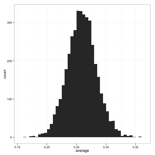
Let’s look at the distribution of batting averages across players.

(For the sake of estimating the prior distribution, I’ve filtered out all players that have fewer than 500 at-bats, since we’ll get a better estimate from the less noisy cases. I show a more principled approach in the Appendix).
The first step of empirical Bayes estimation is to estimate a beta prior using this data. Estimating priors from the data you’re currently analyzing is not the typical Bayesian approach- usually you decide on your priors ahead of time. There’s a lot of debate and discussion about when and where it’s appropriate to use empirical Bayesian methods, but it basically comes down to how many observations we have: if we have a lot, we can get a good estimate that doesn’t depend much on any one individual. Empirical Bayes is an approximation to more exact Bayesian methods- and with the amount of data we have, it’s a very good approximation.
So far, a beta distribution looks like a pretty appropriate choice based on the above histogram. (What would make it a bad choice? Well, suppose the histogram had two peaks, or three, instead of one. Then we might need a mixture of Betas, or an even more complicated model). So we know we want to fit the following model:
\[X\sim\mbox{Beta}(\alpha_0,\beta_0)\]We just need to pick \(\alpha_0\) and \(\beta_0\), which we call “hyper-parameters” of our model. There are many methods in R for fitting a probability distribution to data (optim, mle, bbmle, etc). You don’t even have to use maximum likelihood: you could use the mean and variance, called the “method of moments”. But we’ll use the fitdistr function from MASS.
# just like the graph, we have to filter for the players we actually
# have a decent estimate of
career_filtered <- career %>%
    filter(AB >= 500)

m <- MASS::fitdistr(career_filtered$average, dbeta,
                    start = list(shape1 = 1, shape2 = 10))

alpha0 <- m$estimate[1]
beta0 <- m$estimate[2]
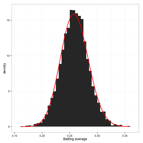
This comes up with \(\alpha_0=78.661\) and \(\beta_0=224.875\). How well does this fit the data?

Not bad! Not perfect, but something we can work with.
Step 2: Use that distribution as a prior for each individual estimate
Now when we look at any individual to estimate their batting average, we’ll start with our overall prior, and update based on the individual evidence. I went over this process in detail in the original Beta distribution post: it’s as simple as adding \(\alpha_0\) to the number of hits, and \(\alpha_0 + \beta_0\) to the total number of at-bats.
For example, consider our hypothetical batter from the introduction that went up 1000 times, and got 300 hits. We would estimate his batting average as:
\[\frac{300+\alpha_0}{1000+\alpha_0+\beta_0}=\frac{300+78.7}{1000+78.7+224.9}=0.29\]How about the batter who went up only 10 times, and got 4 hits. We would estimate his batting average as:
\[\frac{4+\alpha_0}{10+\alpha_0+\beta_0}=\frac{4+78.7}{10+78.7+224.9}=0.264\]Thus, even though \(\frac{4}{10}>\frac{300}{1000}\), we would guess that the \(\frac{300}{1000}\) batter is better than the \(\frac{4}{10}\) batter!
Performing this calculation for all the batters is simple enough:
career_eb <- career %>%
    mutate(eb_estimate = (H + alpha0) / (AB + alpha0 + beta0))
Results
Now we can ask: who are the best batters by this improved estimate?
| name | H | AB | average | eb_estimate |
|---|---|---|---|---|
| Rogers Hornsby | 2930 | 8173 | 0.358 | 0.355 |
| Shoeless Joe Jackson | 1772 | 4981 | 0.356 | 0.350 |
| Ed Delahanty | 2596 | 7505 | 0.346 | 0.343 |
| Billy Hamilton | 2158 | 6268 | 0.344 | 0.340 |
| Harry Heilmann | 2660 | 7787 | 0.342 | 0.339 |
Who are the worst batters?
| name | H | AB | average | eb_estimate |
|---|---|---|---|---|
| Bill Bergen | 516 | 3028 | 0.170 | 0.178 |
| Ray Oyler | 221 | 1265 | 0.175 | 0.191 |
| John Vukovich | 90 | 559 | 0.161 | 0.196 |
| John Humphries | 52 | 364 | 0.143 | 0.196 |
| George Baker | 74 | 474 | 0.156 | 0.196 |
Notice that in each of these cases, empirical Bayes didn’t simply pick the players who had 1 or 2 at-bats. It found players who batted well, or poorly, across a long career. What a load off our minds: we can start using these empirical Bayes estimates in downstream analyses and algorithms, and not worry that we’re accidentally letting \(0/1\) or \(1/1\) cases ruin everything.
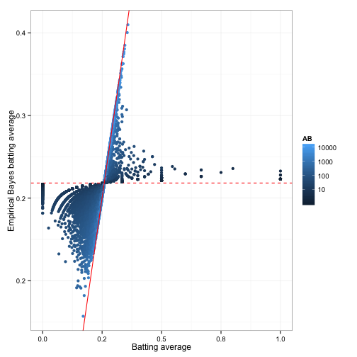
Overall, let’s see how empirical Bayes changed all of the batting average estimates:

The horizontal dashed red line marks \(y=\frac{\alpha_0}{\alpha_0 + \beta_0}=0.259\)- that’s what we would guess someone’s batting average was if we had no evidence at all. Notice that points above that line tend to move down towards it, while points below it move up.
The diagonal red line marks \(x=y\). Points that lie close to it are the ones that didn’t get shrunk at all by empirical Bayes. Notice that they’re the ones with the highest number of at-bats (the brightest blue): they have enough evidence that we’re willing to believe the naive batting average estimate.
This is why this process is sometimes called shrinkage: we’ve moved all our estimates towards the average. How much it moves these estimates depends on how much evidence we have: if we have very little evidence (4 hits out of 10) we move it a lot, if we have a lot of evidence (300 hits out of 1000) we move it only a little. That’s shrinkage in a nutshell: Extraordinary outliers require extraordinary evidence.
Conclusion: So easy it feels like cheating
Recall that there were two steps in empirical Bayes estimation:
- Estimate the overall distribution of your data.
- Use that distribution as your prior for estimating each average.
Step 1 can be done once, “offline”- analyze all your data and come up with some estimates of your overall distribution. Step 2 is done for each new observation you’re considering. You might be estimating the success of a post or an ad, or classifying the behavior of a user in terms of how often they make a particular choice.
And because we’re using the beta and the binomial, consider how easy that second step is. All we did was add one number to the successes, and add another number to the total. You can build that into your production system with a single line of code that takes nanoseconds to run.
// We hired a Data Scientist to analyze our Big Data
// and all we got was this lousy line of code.
float estimate = (successes + 78.7) / (total + 303.5);
That really is so simple that it feels like cheating- like the kind of “fudge factor” you might throw into your code, with the intention of coming back to it later to do some real Machine Learning.
I bring this up to disprove the notion that statistical sophistication necessarily means dealing with complicated, burdensome algorithms. This Bayesian approach is based on sound principles, but it’s still easy to implement. Conversely, next time you think “I only have time to implement a dumb hack,” remember that you can use methods like these: it’s a way to choose your fudge factor. Some dumb hacks are better than others!
But when anyone asks what you did, remember to call it “empirical Bayesian shrinkage towards a Beta prior.” We statisticians have to keep up appearances.
Appendix: How could we make this more complicated?
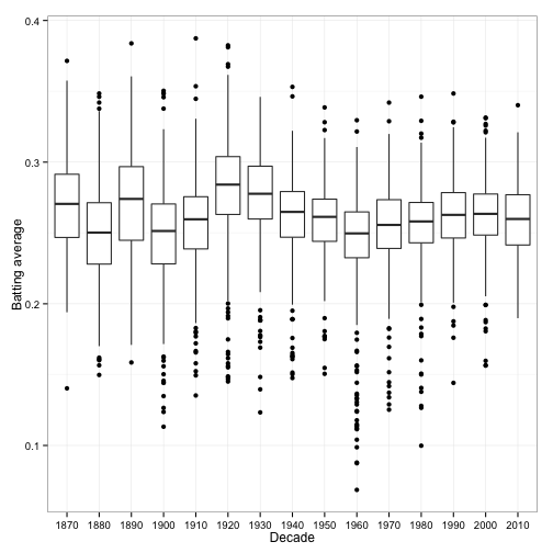
We’ve made some enormous simplifications in this post. For one thing, we assumed all batting averages are drawn from a single distribution. In reality, we’d expect that it depends on some known factors. For instance, the distribution of batting averages has changed over time:

Ideally, we’d want to estimate a different Beta prior for each decade. Similarly, we could estimate separate priors for each team, a separate prior for pitchers, and so on. One useful approach to this is Bayesian hierarchical modeling (as used in, for example, this study of SAT scores across different schools).
Also, as alluded to above, we shouldn’t be estimating the distribution of batting averages using only the ones with more than 500 at-bats. Really, we should use all of our data to estimate the distribution, but give more consideration to the players with a higher number of at-bats. This can be done by fitting a beta-binomial distribution. For instance, we can use the dbetabinom.ab function from VGAM, and the mle function:
library(VGAM)

# negative log likelihood of data given alpha; beta
ll <- function(alpha, beta) {
  -sum(dbetabinom.ab(career$H, career$AB, alpha, beta, log = TRUE))
}

m <- mle(ll, start = list(alpha = 1, beta = 10), method = "L-BFGS-B")
coef(m)
## alpha beta
## 75 222We end up getting almost the same prior, which is reassuring!
