In May, some friends and I built Tagger News, a real-time automatic classifier of Hacker News articles based on their text (see here for more about how we built it). This process started me down some interesting paths, particularly analyzing trends in titles. By finding words that became more or less common in Hacker News titles over time, we can see what topics were gaining or losing interest in the tech world.
I thought I’d share some of these analyses here. As with most of my text analysis posts, I’ll be analyzing it with the tidytext package written by me and Julia Silge. (Check out our soon-to-be-released book on the subject, Text Mining with R!)
Processing one million Hacker News articles
The titles (and dates, and links) of Hacker News articles are helpfully stored on Google Bigquery. We start with a dataset of a million Hacker News article titles, which covers about 3 and a half years of posts. I downloaded it on 2017-06-04 with the following query:
SELECT id, score, time, title, url FROM [bigquery-public-data:hacker_news.full]
  WHERE deleted IS null AND dead IS null AND type = 'story'
  ORDER BY time DESC
  LIMIT 1000000
I’m hosting the dataset so that you can read it yourself (note that it’s a moderately large and compressed file so it may take a minute to read) as follows:
library(tidyverse)
library(lubridate)

stories <- read_csv("http://varianceexplained.org/files/stories_1000000.csv.gz") %>%
  mutate(time = as.POSIXct(time, origin = "1970-01-01"),
         month = round_date(time, "month"))
Whenever we read in a text dataset, the first step is usually to tokenize it (split it up into words) and remove stopwords (like “the” or “and”). As described here, we can do this with tidytext’s unnest_tokens function.
library(tidyverse)
library(tidytext)
library(stringr)

title_words <- stories %>%
  arrange(desc(score)) %>%
  distinct(title, .keep_all = TRUE) %>%
  unnest_tokens(word, title, drop = FALSE) %>%
  distinct(id, word, .keep_all = TRUE) %>%
  anti_join(stop_words, by = "word") %>%
  filter(str_detect(word, "[^\\d]")) %>%
  group_by(word) %>%
  mutate(word_total = n()) %>%
  ungroup()
This creates a pretty large data frame (4443083 rows) with one row per word per post. For example, we could use this to find and visualize the most common words in Hacker News posts during this 3.5 year period.
word_counts <- title_words %>%
  count(word, sort = TRUE)
word_counts %>%
head(25) %>%
mutate(word = reorder(word, n)) %>%
ggplot(aes(word, n)) +
geom_col(fill = "lightblue") +
scale_y_continuous(labels = comma_format()) +
coord_flip() +
labs(title = "Most common words in Hacker News titles",
subtitle = "Among the last million stories; stop words removed",
y = "# of uses")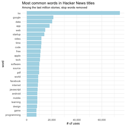
The top result, “hn”, comes from the common constructions of “Show HN” and “Ask HN”, which are often prepended to a title. Among the other words, there’s nothing we wouldn’t have expected from following Hacker News. There some notable technology companies like Google, Apple, and Facebook, along with common topics in tech discussions like “app”, “data” and “startup”.
Change over time
What words and topics have become more frequent, or less frequent, over time? These could give us a sense of the changing technology ecosystem, and let us predict what topics will continue to grow in relevance.
To achieve this, we’ll first count the occurrences of words in titles by month.
stories_per_month <- stories %>%
  group_by(month) %>%
  summarize(month_total = n())

word_month_counts <- title_words %>%
  filter(word_total >= 1000) %>%
  count(word, month) %>%
  complete(word, month, fill = list(n = 0)) %>%
  inner_join(stories_per_month, by = "month") %>%
  mutate(percent = n / month_total) %>%
  mutate(year = year(month) + yday(month) / 365)

word_month_counts
## # A tibble: 33,480 x 6
## word month n month_total percent year
## <chr> <dttm> <dbl> <int> <dbl> <dbl>
## 1 2.0 2013-10-01 42 20542 0.002044592 2013.751
## 2 2.0 2013-11-01 55 23402 0.002350226 2013.836
## 3 2.0 2013-12-01 26 21945 0.001184780 2013.918
## 4 2.0 2014-01-01 25 19186 0.001303033 2014.003
## 5 2.0 2014-02-01 31 22295 0.001390446 2014.088
## 6 2.0 2014-03-01 37 21118 0.001752060 2014.164
## 7 2.0 2014-04-01 33 23673 0.001393993 2014.249
## 8 2.0 2014-05-01 28 21394 0.001308778 2014.332
## 9 2.0 2014-06-01 47 19265 0.002439657 2014.416
## 10 2.0 2014-07-01 25 19829 0.001260780 2014.499
## # ... with 33,470 more rowsWe can then use my broom package to fit a model (logistic regression) to examine whether the frequency of each word is increasing or decreasing over time. Every term will then have a growth rate (as an exponential term) associated with it.
library(broom)

mod <- ~ glm(cbind(n, month_total - n) ~ year, ., family = "binomial")

slopes <- word_month_counts %>%
  nest(-word) %>%
  mutate(model = map(data, mod)) %>%
  unnest(map(model, tidy)) %>%
  filter(term == "year") %>%
  arrange(desc(estimate))

slopes
## # A tibble: 744 x 6
## word term estimate std.error statistic p.value
## <chr> <chr> <dbl> <dbl> <dbl> <dbl>
## 1 trump year 1.7570144 0.04052662 43.35458 0.000000e+00
## 2 ai year 0.7830541 0.01756776 44.57335 0.000000e+00
## 3 blockchain year 0.6557110 0.02682345 24.44544 5.626574e-132
## 4 neural year 0.6270933 0.02617919 23.95388 8.418336e-127
## 5 react year 0.6027489 0.01628292 37.01725 6.045233e-300
## 6 vr year 0.5260498 0.02247906 23.40177 4.099556e-121
## 7 bot year 0.5178669 0.02600166 19.91669 2.916460e-88
## 8 iot year 0.5076088 0.02514613 20.18636 1.290270e-90
## 9 microservices year 0.4933223 0.03180060 15.51299 2.833910e-54
## 10 slack year 0.4718030 0.02287605 20.62432 1.660491e-94
## # ... with 734 more rowsWe can now ask: what terms have been increasing in frequency in Hacker News titles?
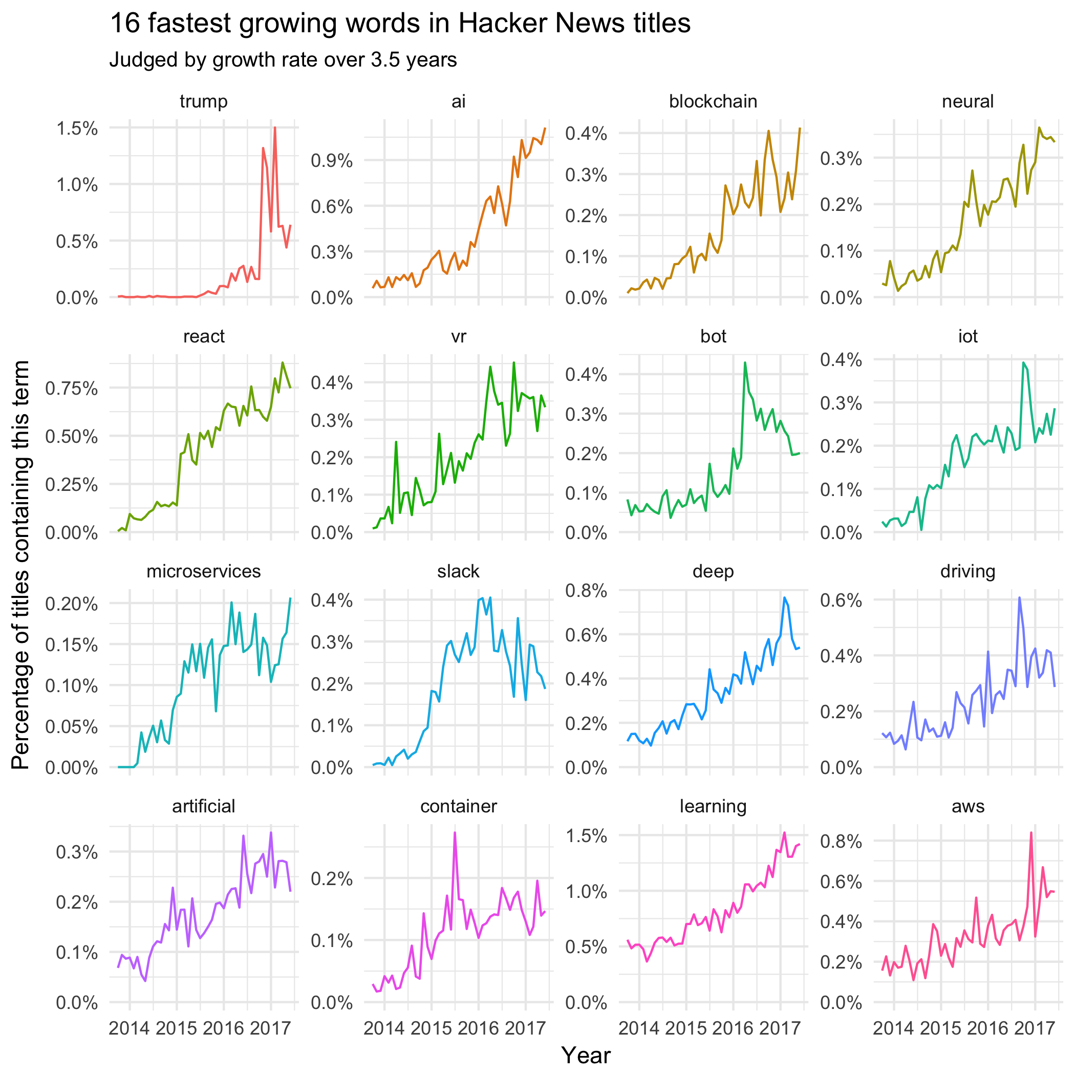
It makes sense that “Trump” is the word that’s growing most quickly. While it shows a moderate growth after Trump announced his candidacy in mid-2015, it shows a sharp increase around the time of the 2016 election (though it hasn’t been quite as dominant in the months since his inauguration). The next fastest growing terms include “AI” and “blockchain”, both topics that have shown a recent surge of interest. (We can also see “machine learning”, “AWS”, and “bot” among the growing terms).
What words have been decreasing in frequency in Hacker News titles?
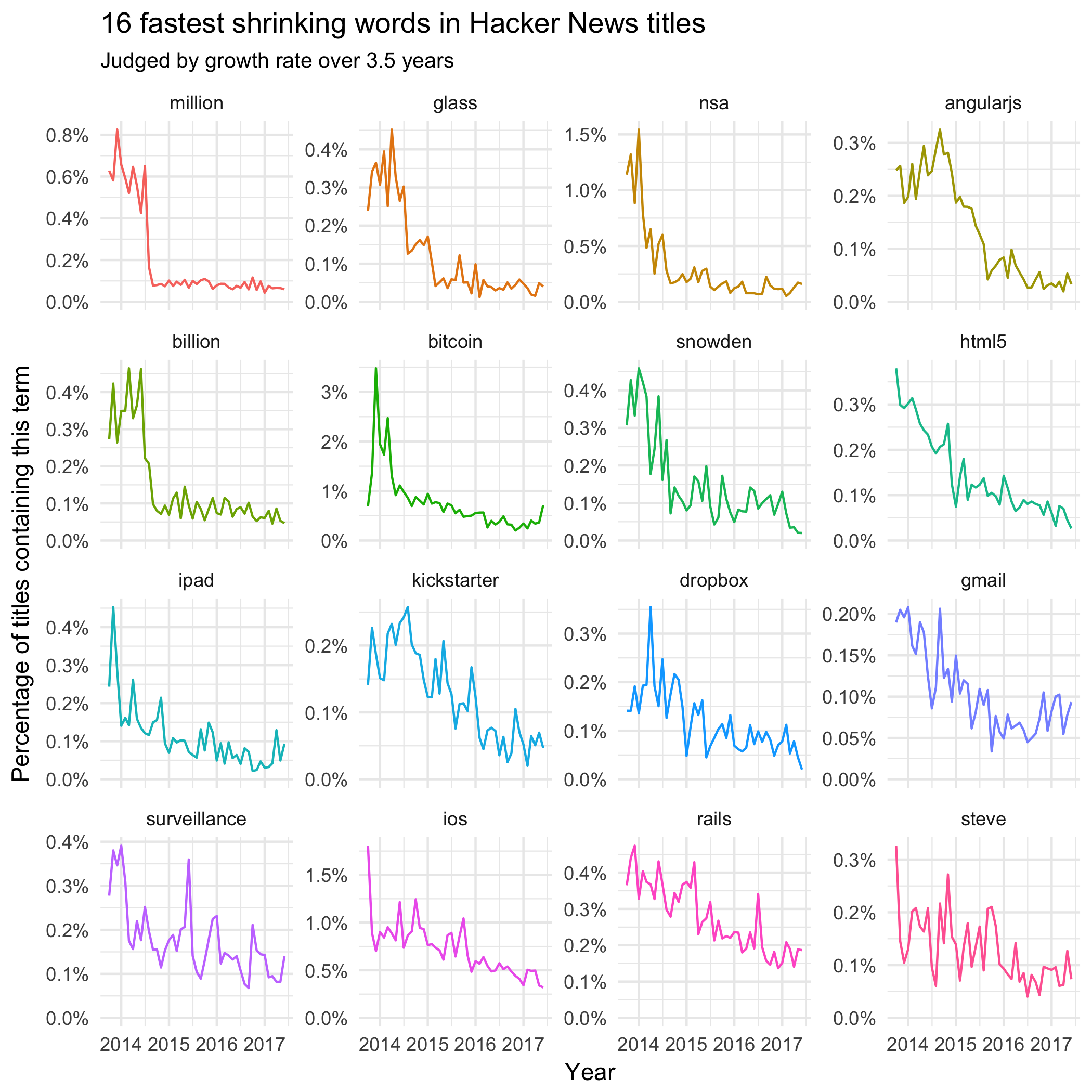
This shows a few topics in which interest has died out since 2013, including Google Glass and Gmail. Discussion of Edward Snowden and the NSA was fresh news around 2013-2014, so it makes sense that it’s declined since. There are also some notable technologies that people write about less, such as AngularJS, HTML5, and Ruby on Rails. It’s interesting to compare these to Stack Overflow Trends during that time period, in which AngularJS has been growing in terms of Stack Overflow questions asked (HTML5 and Rails have leveled off). It’s possible that discussion on HN is a “leading indicator”, showing a surge articles when a technology first gets popular.
(I don’t currently have a guess for why “million” and “billion” had sudden dropoffs in 2014. Is it some artifact of the Hacker News policy, with the word becoming edited or deleted in newer posts? Or is it a real change in what the site discusses?)
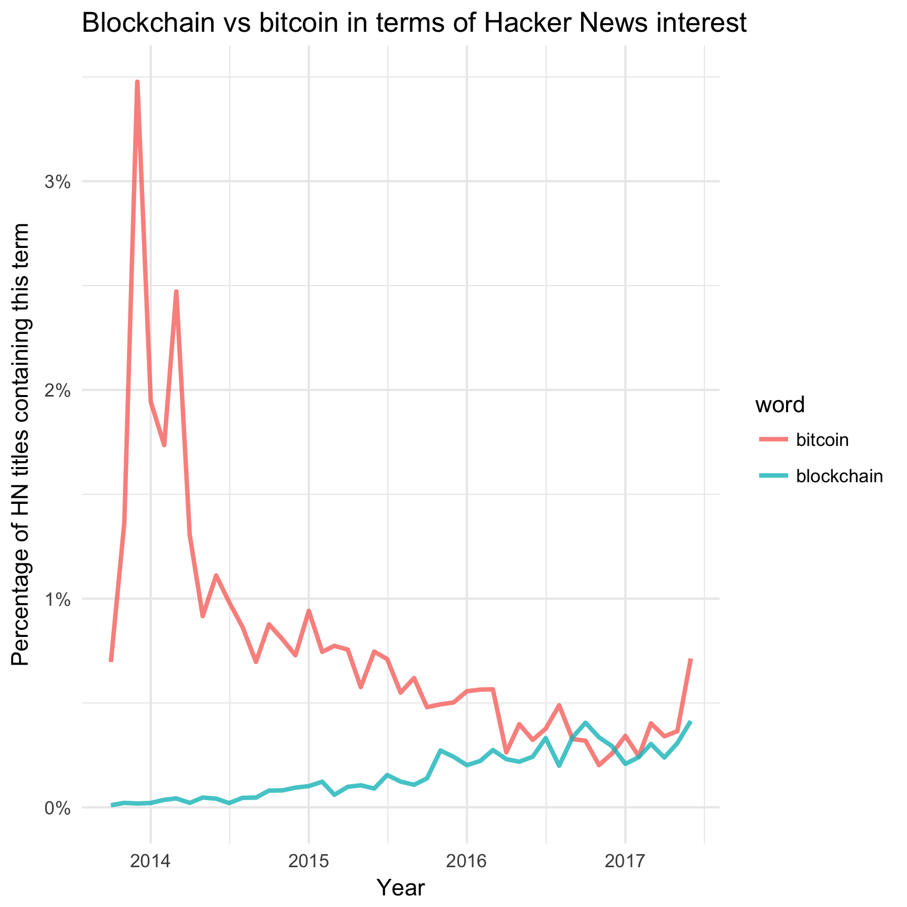
Interestingly, the conversation around “bitcoin” peaked around 2013-2014 (with a recent uptick due to a surge in Bitcoin’s price), while discussion of the blockchain has been growing in the years since. Comparing them on the same axes makes in clear that the blockchain has roughly “caught up to” bitcoin in terms of general interest:
Words that passed their peak
We can learn a lot by examining words , but we’re misses an important piece of the puzzle: there are some words that grew in interest for part of this time, then “passed their peak.” This is more complicated to explore quantitatively, but one approach is to find words where the ratio of the peak in the trend to the average is especially high. To reduce the effect of random noise, we use a cubic spline to smooth each trend before determining the peak.
library(splines)

mod2 <- ~ glm(cbind(n, month_total - n) ~ ns(year, 4), ., family = "binomial")

# Fit a cubic spline to each shape
spline_predictions <- word_month_counts %>%
  mutate(year = as.integer(as.Date(month)) / 365) %>%
  nest(-word) %>%
  mutate(model = map(data, mod2)) %>%
  unnest(map2(model, data, augment, type.predict = "response"))

# Find the terms with the highest peak / average ratio
peak_per_month <- spline_predictions %>%
  group_by(word) %>%
  mutate(average = mean(.fitted)) %>%
  top_n(1, .fitted) %>%
  ungroup() %>%
  mutate(ratio = .fitted / average) %>%
  filter(month != min(month), month != max(month)) %>%
  top_n(16, ratio)
Here are 16 terms that had strong peaks at various point in the last 3.5 years.
peak_per_month %>%
  select(word, peak = month) %>%
  inner_join(spline_predictions, by = "word") %>%
  mutate(word = reorder(word, peak)) %>%
  ggplot(aes(month, percent)) +
  geom_line(aes(color = word), show.legend = FALSE) +
  geom_line(aes(y = .fitted), lty = 2) +
  facet_wrap(~ word, scales = "free_y") +
  scale_y_continuous(labels = percent_format()) +
  expand_limits(y = 0) +
  labs(x = "Year",
       y = "Percent of titles containing this term",
       title = "16 words that peaked then declined in Hacker News titles",
       subtitle = "Spline fit (df = 4) shown.\nSelected based on the peak of the spline divided by the overall average; ordered by peak month.")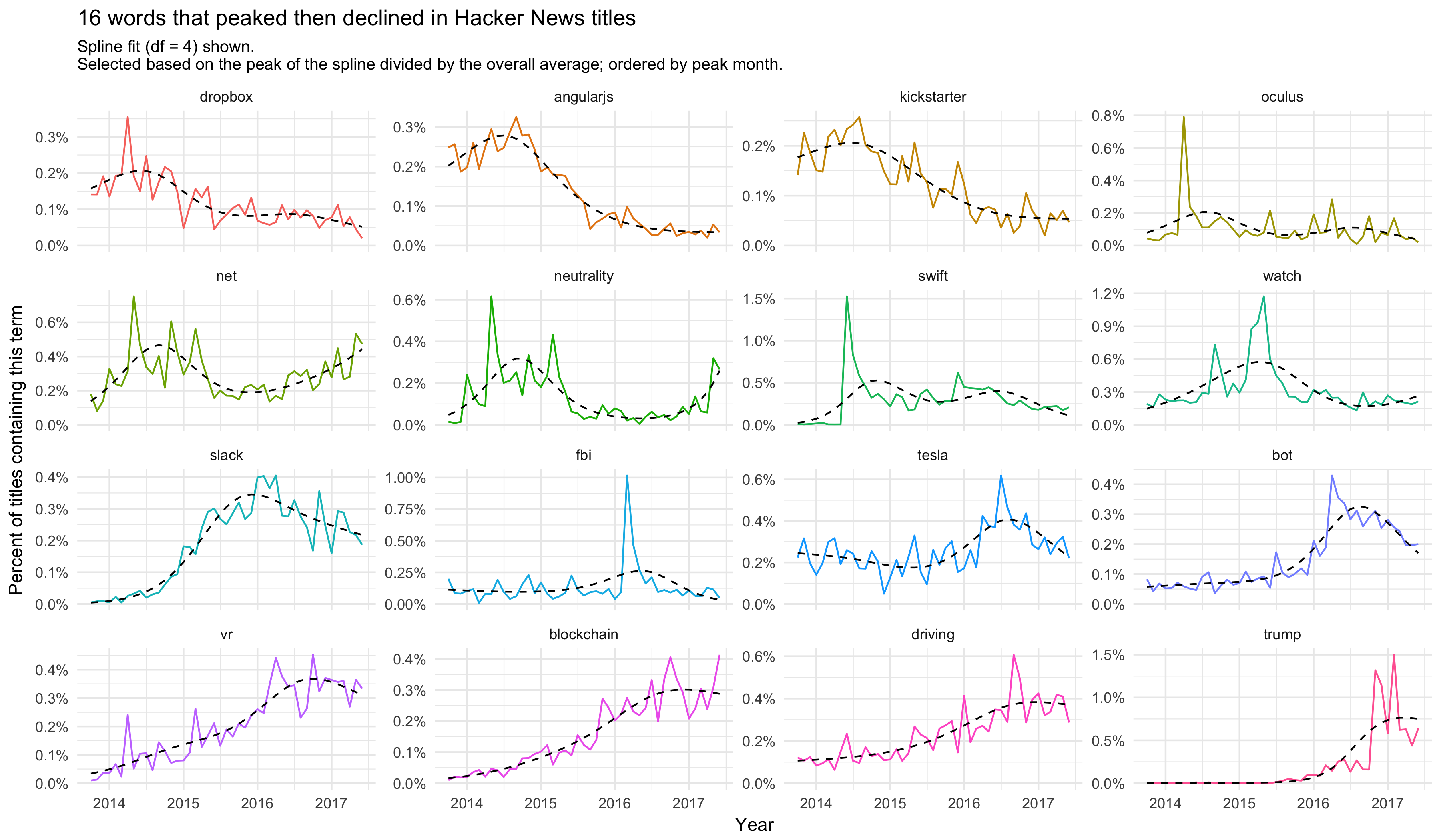
We can see a peak of discussion around net neutrality in 2015 (though it’s shown a recent resurgence of interest). You can spot the introduction of Swift and the Apple Watch, then a moderate decline in discussion around them, and there are sudden jolts of discussion around Oculus in 2014 (with Facebook’s purchase of the company) and the FBI in 2016 (news around Clinton’s email server). The graph suggests the discussion around Slack, bots, Tesla, and virtual reality may have leveled off (though in some cases it may be too early to tell).
What’s next
I have some more analyses of Hacker News posts I’ll be sharing in the future, including analyses of word correlations, examination of what words and topics tend to get upvoted, and some improvements on the Tagger News classification algorithm. The series will also give me the chance to highlight more techniques from Text Mining with R, including word networks and topic modeling.
