Twitter has seen a recent trend of “first 7” and “favorite 7” hashtags, like #7FirstJobs and #7FavFilms. Last week I added one to the mix, about my 7 favorite R packages:
devtools
— David Robinson (@drob) August 16, 2016
dplyr
ggplot2
knitr
Rcpp
rmarkdown
shiny#7FavPackages #rstats
Hadley Wickham agreed to share his own, but on one condition:
@drob I'll do it if you write a script to scrape the tweets, plot overall most common, and common co-occurences
— Hadley Wickham (@hadleywickham) August 16, 2016
Hadley followed through, so now it’s my turn.
Setup
We can use the same twitteR package that I used in my analysis of Trump’s Twitter account:
library(twitteR)
library(purrr)
library(dplyr)
library(stringr)

# You'd need to set up authentication before running this
# See help(setup_twitter_oauth)
tweets <- searchTwitter("#7FavPackages", n = 3200) %>%
  map_df(as.data.frame)

# Grab only the first for each user (some had followups), and ignore retweets
tweets <- tweets %>%
  filter(!str_detect(text, "^RT ")) %>%
  arrange(created) %>%
  distinct(screenName, .keep_all = TRUE)
There were 116 (unique) tweets in this hashtag. I can use the tidytext package to analyze them, using a custom regular expression.
library(BiocInstaller)
# to avoid non-package words
built_in <- tolower(sessionInfo()$basePkgs)
cran_pkgs <- tolower(rownames(available.packages()))
bioc_pkgs <- tolower(rownames(available.packages(repos = biocinstallRepos()[1:3])))
blacklist <- c("all")
library(tidytext)
spl_re <- "[^a-zA-Z\\d\\@\\#\\.]"
link_re <- "https://t.co/[A-Za-z\\d]+|&"
packages <- tweets %>%
mutate(text = str_replace_all(text, link_re, "")) %>%
unnest_tokens(package, text, token = "regex", pattern = spl_re) %>%
filter(package %in% c(cran_pkgs, bioc_pkgs, built_in)) %>%
distinct(id, package) %>%
filter(!package %in% blacklist)
pkg_counts <- packages %>%
count(package, sort = TRUE)Note that since a lot of non-package words got mixed in with these tweets, I filtered for only packages in CRAN and Bioconductor (so packages that are only on GitHub or elsewhere won’t be included, though anecdotally I didn’t notice any among the tweets). Tweeters were sometimes inconsistent about case as well, so I kept all packages lowercase throughout this analysis.
General results
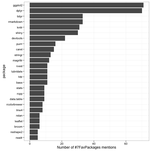
There were 700 occurrences of 184 packages in these tweets. What were the most common?
Some observations:
- ggplot2 and dplyr were the most popular packages, each mentioned by more than half the tweets, and other packages by Hadley like tidyr, devtools, purrr and stringr weren’t far behind. This isn’t too surprising, since much of the attention to the hashtag came with Hadley’s tweet.
@drob @JaySun_Bee @ma_salmon HOW IS THAT BIASED?
— Hadley Wickham (@hadleywickham) August 16, 2016
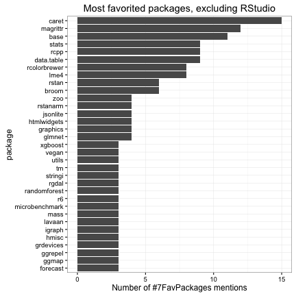
- The next most popular packages involved reproducible research (rmarkdown and knitr), along with other RStudio tools like shiny. What if I excluded packages maintained by RStudio (or RStudio employees like Hadley and Yihui)?
- The vast majority of packages people listed as their favorite were CRAN packages: only 7 Bioconductor packages were mentioned (though it’s worth noting they occurred across four different tweets):
packages %>%
  filter(package %in% bioc_pkgs)
## # A tibble: 7 x 2
## id package
## <chr> <chr>
## 1 765622260556238848 xcms
## 2 765637117976387584 edger
## 3 765637117976387584 limma
## 4 765669197284245504 biomart
## 5 765669197284245504 genomicranges
## 6 765669197284245504 deseq2
## 7 765630231948308481 genefilter- There were 109 CRAN packages that were mentioned only once, and those showed a rather large variety. A random sample of 10:
set.seed(2016)
pkg_counts %>%
  filter(n == 1, !package %in% bioc_pkgs) %>%
  sample_n(10)
## # A tibble: 10 x 2
## package n
## <chr> <int>
## 1 fclust 1
## 2 dt 1
## 3 shinystan 1
## 4 domc 1
## 5 mapview 1
## 6 daff 1
## 7 pbapply 1
## 8 visnetwork 1
## 9 af 1
## 10 arm 1Correlations
What packages tend to be “co-favorited”- that is, listed by the same people? Here I’m using my in-development widyr package, which makes it easy to calculate pairwise correlations in a tidy data frame.
# install with devtools::install_github("dgrtwo/widyr")
library(widyr)

# use only packages with at least 4 mentions, to reduce noise
pkg_counts <- packages %>%
  count(package) %>%
  filter(n >= 4)

pkg_correlations <- packages %>%
  semi_join(pkg_counts) %>%
  pairwise_cor(package, id, sort = TRUE, upper = FALSE)

pkg_correlations
## # A tibble: 465 x 3
## item1 item2 correlation
## <chr> <chr> <dbl>
## 1 base graphics 0.5813129
## 2 graphics stats 0.4716609
## 3 base stats 0.4495913
## 4 dplyr tidyr 0.3822511
## 5 rstan rstanarm 0.3791074
## 6 dplyr ggplot2 0.3483315
## 7 ggplot2 knitr 0.3032979
## 8 dplyr shiny 0.3027743
## 9 data.table htmlwidgets 0.2937083
## 10 ggplot2 tidyr 0.2811096
## # ... with 455 more rowsFor instance, this shows the greatest correlation (technically a phi coefficient) were between the base, graphics, and stats packages, by people showing loyalty to built in packages.
I like using the ggraph package to visualize these relationships:
library(ggraph)
library(igraph)

set.seed(2016)

# we set an arbitrary threshold of connectivity
pkg_correlations %>%
  filter(correlation > .2) %>%
  graph_from_data_frame(vertices = pkg_counts) %>%
  ggraph(layout = "fr") +
  geom_edge_link(aes(edge_alpha = correlation)) +
  geom_node_point(aes(size = n), color = "lightblue") +
  theme_void() +
  geom_node_text(aes(label = name), repel = TRUE) +
  theme(legend.position = "none")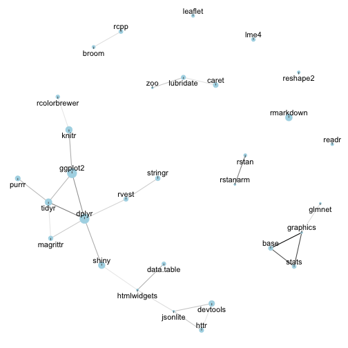
You can recognize most of RStudio’s packages (ggplot2, dplyr, tidyr, knitr, shiny) in the cluster on the bottom left of the graph. At the bottom right you can see the “base” cluster (stats, base, utils, grid, graphics), with people who showed their loyalty to base packages.
Beyond that, the relationships are a bit harder to parse (outside of some expected combinations like rstan and rstanarm): we may just not have enough data to create reliable correlations.
Compared to CRAN dependencies
This isn’t a particularly scientific survey, to say the least. So how does it compare to another metric of a package’s popularity: the number of packages that Depend, Import, or Suggest it on CRAN? (You could also compare to # of CRAN downloads using the cranlogs package, but since most downloads are due to dependencies, the two metrics give rather similar results).
We can discover this using the available.packages() function, along with some processing.
library(tidyr)

pkgs <- available.packages() %>%
  as.data.frame() %>%
  tbl_df()

requirements <- pkgs %>%
  unite(Requires, Depends, Imports, Suggests, sep = ",") %>%
  transmute(Package = as.character(Package),
            Requires = as.character(Requires)) %>%
  unnest(Requires = str_split(Requires, ",")) %>%
  mutate(Requires = str_replace(Requires, "\n", "")) %>%
  mutate(Requires = str_trim(str_replace(Requires, "\\(.*", ""))) %>%
  filter(!(Requires %in% c("R", "NA", "", built_in)))

requirements
## # A tibble: 34,781 x 2
## Package Requires
## <chr> <chr>
## 1 A3 xtable
## 2 A3 pbapply
## 3 A3 randomForest
## 4 A3 e1071
## 5 abbyyR httr
## 6 abbyyR XML
## 7 abbyyR curl
## 8 abbyyR readr
## 9 abbyyR progress
## 10 abbyyR testthat
## # ... with 34,771 more rowspackage_info <- requirements %>%
count(Package = Requires) %>%
rename(NRequiredBy = n) %>%
left_join(count(requirements, Package)) %>%
rename(NRequires = n) %>%
replace_na(list(NRequires = 0))
package_info## # A tibble: 2,925 x 3
## Package NRequiredBy NRequires
## <chr> <int> <dbl>
## 1 a4Base 1 0
## 2 a4Core 1 0
## 3 abc 3 5
## 4 abc.data 2 0
## 5 abd 1 12
## 6 abind 95 0
## 7 AcceptanceSampling 1 0
## 8 acepack 2 0
## 9 acp 1 2
## 10 acs 3 4
## # ... with 2,915 more rowsWe can compare the number of mentions in the hashtag to the number of pacakges:
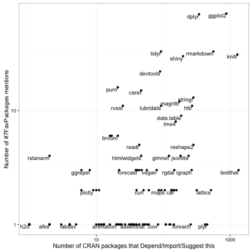
Some like dplyr, ggplot2, and knitr are popular both within the hashtag and as CRAN dependencies. Some relatively new packages like purrr are popular on Twitter but haven’t built up as many packages needing them, and others like plyr and foreach are a common dependency but are barely mentioned. (This isn’t even counting the many packages never mentioned in the hashtag).
Since we have this dependency data, I can’t resist looking for correlations just like we did with the hashtag data. What packages tend to be depended on together?
## # A tibble: 64,770 x 3
##            item1         item2 correlation
##            <chr>         <chr>       <dbl>
## 1           R.oo   R.methodsS3   0.9031741
## 2    R.methodsS3          R.oo   0.9031741
## 3     doParallel       foreach   0.7341718
## 4        foreach    doParallel   0.7341718
## 5       timeDate    timeSeries   0.7084369
## 6     timeSeries      timeDate   0.7084369
## 7  gWidgetsRGtk2      gWidgets   0.6974373
## 8       gWidgets gWidgetsRGtk2   0.6974373
## 9           ergm       network   0.6336521
## 10       network          ergm   0.6336521
## # ... with 64,760 more rows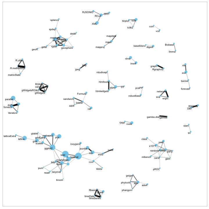
(I skipped the code for these, but you can find it all here).
Some observations from the full network (while it’s not related to the hashtag, still quite interesting):
- The RStudio cluster is prominent in the lower left, with ggplot2, knitr and testthat serving as the core anchors. A lot of packages depend on these in combination.
- You can spot a tight cluster of spatial statistics packages in the upper left (around “sp”) and of machine learning packages near the bottom right (around caret, rpart, and nnet)
- Smaller clusters include parallelization on the left (parallel, doParallel), time series forecasting on the upper right (zoo, xts, forecast), and parsing API data on top (RCurl, rjson, XML)
One thing I like about this 2D layout (much as I’ve done with programming languages using Stack Overflow data) is that we can bring in our hashtag information, and spot visually what types of packages tended to be favorited.
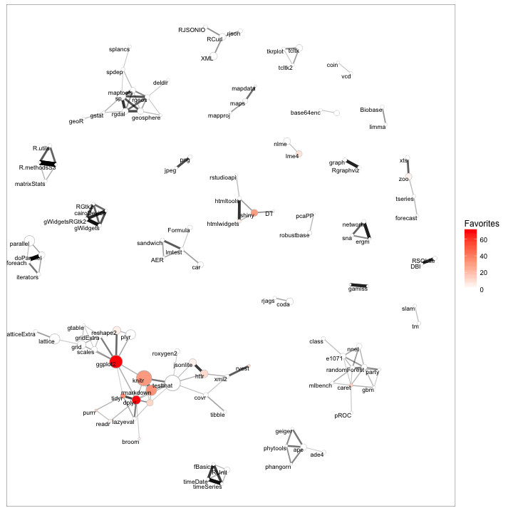
This confirms our observation that the favorited packages are slanted towards the tidyverse/RStudio cluster.
The #7First and #7Fav hashtags have been dying down a bit, but it may still be interesting to try this analysis for others, especially ones with more activity. Maëlle Salmon is working on a great analysis of #7FirstJobs and I’m sure others would be informative.
