
This year, more than fifty thousand programmers answered the Stack Overflow 2016 Developer Survey, in the largest survey of professional developers in history.
Last week Stack Overflow released the full (anonymized) results of the survey at stackoverflow.com/research. To make analysis in R even easier, today I’m also releasing the stacksurveyr package, which contains:
- The full survey results as a processed data frame (
stack_survey) - A data frame with the survey’s schema, including the original text of each question (
stack_schema) - A function that works easily with multiple-response questions (
stack_multi)
This makes it easier than ever to explore this rich dataset and answer questions about the world’s developers.
Examples: Basic exploration
I’ll give a few examples of survey analyses using the dplyr package. For instance, you could discover the most common occupations of survey respondents:
library(stacksurveyr)
library(dplyr)

stack_survey %>%
  count(occupation, sort = TRUE)
## # A tibble: 28 x 2
## occupation n
## <chr> <int>
## 1 Full-stack web developer 13886
## 2 <NA> 6511
## 3 Back-end web developer 6061
## 4 Student 5619
## 5 Desktop developer 3390
## 6 Front-end web developer 2873
## 7 other 2585
## 8 Enterprise level services developer 1471
## 9 Mobile developer - Android 1462
## 10 Mobile developer 1373
## # ... with 18 more rowsWe can also use group_by and summarize to find the highest paid (on average) occupations:
salary_by_occupation <- stack_survey %>%
  filter(occupation != "other") %>%
  group_by(occupation) %>%
  summarize(average_salary = mean(salary_midpoint, na.rm = TRUE)) %>%
  arrange(desc(average_salary))

salary_by_occupation
## # A tibble: 26 x 2
## occupation average_salary
## <chr> <dbl>
## 1 Executive (VP of Eng., CTO, CIO, etc.) 103073.93
## 2 Engineering manager 101047.08
## 3 Enterprise level services developer 79855.62
## 4 DevOps 68731.96
## 5 Product manager 68598.62
## 6 Growth hacker 67878.79
## 7 Machine learning developer 67041.80
## 8 Data scientist 66508.75
## 9 Business intelligence or data warehousing expert 65660.92
## 10 Developer with a statistics or mathematics background 65625.76
## # ... with 16 more rowsThis can be visualized in a bar plot:
library(ggplot2)
library(scales)

salary_by_occupation %>%
  mutate(occupation = reorder(occupation, average_salary)) %>%
  ggplot(aes(occupation, average_salary)) +
  geom_bar(stat = "identity") +
  ylab("Average salary (USD)") +
  scale_y_continuous(labels = dollar_format()) +
  coord_flip()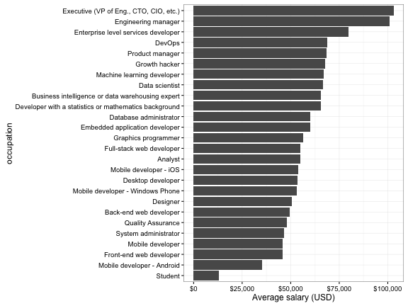
Examples: Multi-response answers
10 of the questions allow multiple responses, as can be noted in the stack_schema variable:
stack_schema %>%
  filter(type == "multi")
## # A tibble: 10 x 4
## column type
## <chr> <chr>
## 1 self_identification multi
## 2 tech_do multi
## 3 tech_want multi
## 4 dev_environment multi
## 5 education multi
## 6 new_job_value multi
## 7 how_to_improve_interview_process multi
## 8 star_wars_vs_star_trek multi
## 9 developer_challenges multi
## 10 why_stack_overflow multi
## # ... with 2 more variables: question <chr>, description <chr>In these cases, the responses are given delimited by ; . Often, these columns are easier to work with and analyze when they are “unnested” into one user-answer pair per row. The package provides the stack_multi function as a shortcut for that unnesting. For example, consider the tech_do column (““Which of the following languages or technologies have you done extensive development with in the last year?”):
stack_multi("tech_do")## # A tibble: 225,075 x 3
## respondent_id column answer
## <int> <chr> <chr>
## 1 4637 tech_do iOS
## 2 4637 tech_do Objective-C
## 3 31743 tech_do Android
## 4 31743 tech_do Arduino / Raspberry Pi
## 5 31743 tech_do AngularJS
## 6 31743 tech_do C
## 7 31743 tech_do C++
## 8 31743 tech_do C#
## 9 31743 tech_do Cassandra
## 10 31743 tech_do CoffeeScript
## # ... with 225,065 more rowsUsing this data, we could find the most common answers:
stack_multi("tech_do") %>%
  count(tech = answer, sort = TRUE)
## # A tibble: 42 x 2
## tech n
## <chr> <int>
## 1 JavaScript 27385
## 2 SQL 21976
## 3 Java 17942
## 4 C# 15283
## 5 PHP 12780
## 6 Python 12282
## 7 C++ 9589
## 8 SQL Server 9306
## 9 AngularJS 8823
## 10 Android 8601
## # ... with 32 more rowsWe can join this with the stack_survey dataset using the respondent_id column. For example, we could look at the most common development technologies used by data scientists:
stack_survey %>%
  filter(occupation == "Data scientist") %>%
  inner_join(stack_multi("tech_do"), by = "respondent_id") %>%
  count(answer, sort = TRUE)
## # A tibble: 42 x 2
## answer n
## <chr> <int>
## 1 Python 507
## 2 SQL 356
## 3 R 352
## 4 Java 240
## 5 JavaScript 207
## 6 C++ 155
## 7 C 125
## 8 Hadoop 108
## 9 SQL Server 98
## 10 Spark 97
## # ... with 32 more rowsOr we could find out the average age and salary of people using each technology, and compare them:
stack_survey %>%
  inner_join(stack_multi("tech_do")) %>%
  group_by(answer) %>%
  summarize_each(funs(mean(., na.rm = TRUE)), age_midpoint, salary_midpoint) %>%
  ggplot(aes(age_midpoint, salary_midpoint)) +
  geom_point() +
  geom_text(aes(label = answer), vjust = 1, hjust = 1) +
  xlab("Average age of people using this technology") +
  ylab("Average salary (USD)") +
  scale_y_continuous(labels = dollar_format())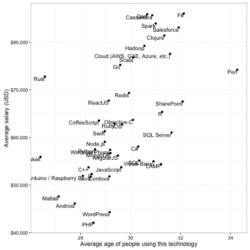
If we want to be a bit more adventurous, we can use the (in-development) widyr package to find correlations among technologies, and the ggraph package to display them as a network of related technologies:
library(widyr)
library(ggraph)
library(igraph)

set.seed(2016)

stack_multi("tech_do") %>%
  pairwise_cor(answer, respondent_id) %>%
  filter(correlation > .15) %>%
  graph_from_data_frame() %>%
  ggraph(layout = "fr") +
  geom_edge_link(aes(edge_alpha = correlation, edge_width = correlation)) +
  geom_node_point(color = "lightblue", size = 7) +
  geom_node_text(aes(label = name), repel = TRUE) +
  theme_void()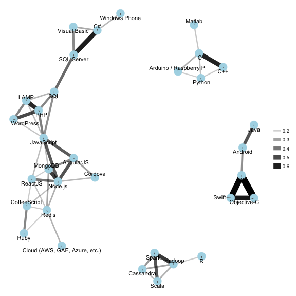
Try the data out for yourself!