
I recently came across a great natural language dataset from Mark Riedel: 112,000 plots of stories downloaded from English language Wikipedia. This includes books, movies, TV episodes, video games- anything that has a Plot section on a Wikipedia page.
This offers a great opportunity to analyze story structure quantitatively. In this post I’ll do a simple analysis, examining what words tend to occur at particular points within a story, including words that characterize the beginning, middle, or end.
As I usually do for text analysis, I’ll be using the tidytext package Julia Silge and I developed last year. To learn more about analyzing datasets like this, see our online book Text Mining with R: A Tidy Approach, soon to be published by O’Reilly. I’ll provide code for the text mining sections so you can follow along. I don’t show the code for most of the visualizations to keep the post concise, but as with all of my posts the code can be found here on GitHub.
Setup
I downloaded and unzipped the plots.zip file from the link on the GitHub repository. We then read the files into R, and combined them using dplyr.
library(readr)
library(dplyr)

# Plots and titles are in separate files
plots <- read_lines("~/Downloads/plots/plots", progress = FALSE)
titles <- read_lines("~/Downloads/plots/titles", progress = FALSE)

# Each story ends with an <EOS> line
plot_text <- data_frame(text = plots) %>%
  mutate(story_number = cumsum(text == "<EOS>") + 1,
         title = titles[story_number]) %>%
  filter(text != "<EOS>")
We can then use the tidytext package to unnest the plots into a tidy format, with one token per line.
library(tidytext)
plot_words <- plot_text %>%
unnest_tokens(word, text)plot_words## # A tibble: 40,330,086 × 3
## story_number title word
## <dbl> <chr> <chr>
## 1 1 Animal Farm old
## 2 1 Animal Farm major
## 3 1 Animal Farm the
## 4 1 Animal Farm old
## 5 1 Animal Farm boar
## 6 1 Animal Farm on
## 7 1 Animal Farm the
## 8 1 Animal Farm manor
## 9 1 Animal Farm farm
## 10 1 Animal Farm summons
## # ... with 40,330,076 more rowsThis dataset contains over 40 million words across 112,000 stories.
Words at the beginning or end of stories
Joseph Campbell introduced the idea of a “hero’s journey”, that every story follows the same structure. Whether or not you buy into his theory, you can agree it’d be surprising if a plot started with a climactic fight, or ended by introducing new characters.
That structure is reflected quantitatively in what words are used at which point in a story: there are some words you’d expect would appear at the start, and others at the end.
As a simple measure of where a word occurs within a plot, we’ll record the median position of each word, along with the number of times it appears.
word_averages <- plot_words %>%
  group_by(title) %>%
  mutate(word_position = row_number() / n()) %>%
  group_by(word) %>%
  summarize(median_position = median(word_position),
            number = n())
We’re not interested in rare words that occurred in only a few plot descriptions, so we’ll filter for ones occurring at least 2,500 times.
word_averages %>%
  filter(number >= 2500) %>%
  arrange(median_position)
## # A tibble: 1,640 × 3
## word median_position number
## <chr> <dbl> <int>
## 1 fictional 0.1193618 2688
## 2 year 0.2013554 18692
## 3 protagonist 0.2029450 3222
## 4 century 0.2096774 3583
## 5 wealthy 0.2356817 5686
## 6 opens 0.2408638 7319
## 7 california 0.2423856 2656
## 8 angeles 0.2580645 2889
## 9 los 0.2661747 3110
## 10 student 0.2692308 6961
## # ... with 1,630 more rowsFor example, we can see that the word “fictional” was used about 2700 times, and that half of its uses were before the 12% mark of the story: it’s highly shifted towards the beginning.
What were were the words most shifted towards the beginning or end of a story?
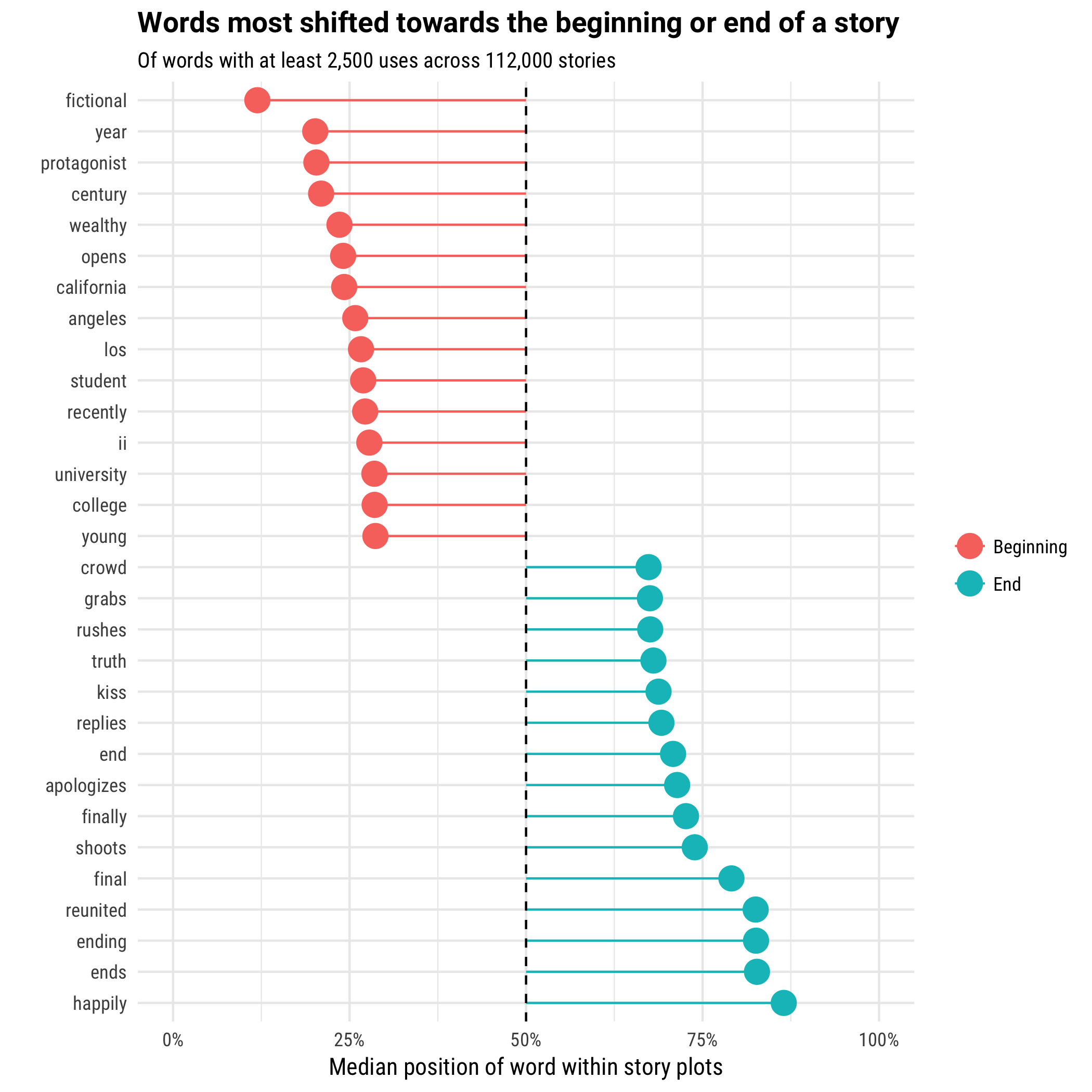
The words shifted towards the beginning of a story tend to describe a setting: “The story opens on the protagonist, a wealthy young 19th century student recently graduated from the fictional University College in Los Angeles, California.”. Most are therefore nouns and adjectives that can be used to specify and describe a person, location, or time period.
In contrast, the words shifted towards the end of a story are packed with excitement! There are a few housekeeping terms you’d expect to find at the end of a plot description (“ending”, “final”), but also a number of verbs suggestive of a climax. “The hero shoots the villain and rushes to the heroine, and apologizes. The two reunited, they kiss.”
Visualizing trends of words
The median gives us a useful summary statistic of where a word appears within a story, but let’s take a closer look at a few. First we’ll divide each story into deciles (first 10%, second 10%, etc), and count the appearances of each word within each decile.
decile_counts <- plot_words %>%
  group_by(title) %>%
  mutate(word_position = row_number() / n()) %>%
  ungroup() %>%
  mutate(decile = ceiling(word_position * 10) / 10) %>%
  count(decile, word)
This lets us visualize the frequency of a word across the length of plot descriptions. We may want to look at the most extreme start/end ones:
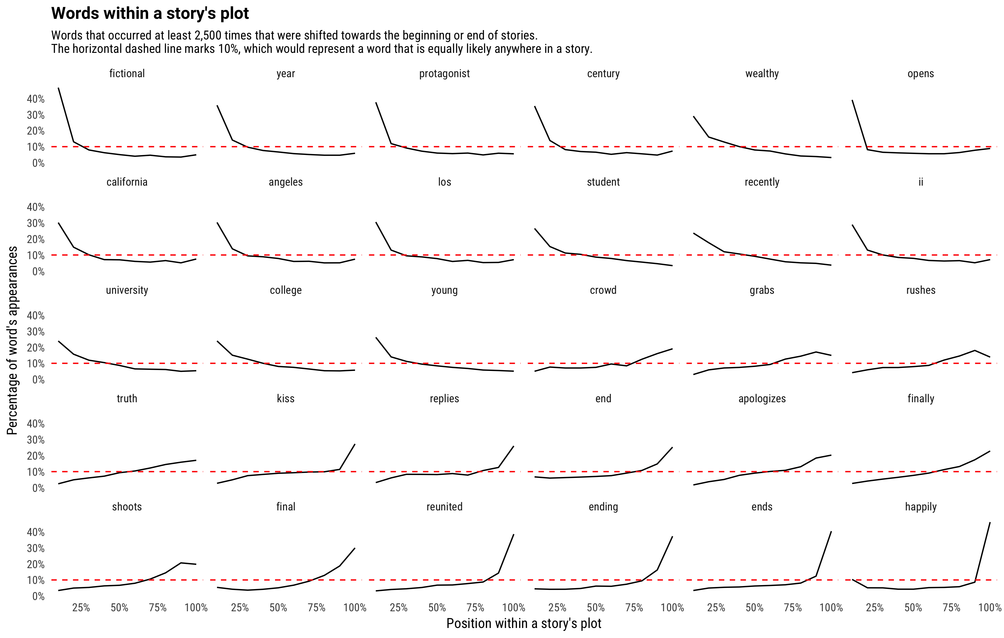
No word happens exclusively at the start or end of a story. Some, like “happily”, remain steady throughout and then spike up at the end (“lived happily ever after”). Other words, like “truth”, or “apologizes”, show a constant rise in frequency over the course of the story, which makes sense: a character generally wouldn’t “apologize” or “realize the truth” right at the start of the story. Similarly, words that establish settings like “wealthy” become steadily rarer the course of the story, as it becomes less likely the plot will introduce new characters.
One interesting feature of the above graph is that while most words peak either at the beginning or end, words like “grabs”, “rushes”, and “shoots” were most common at the 90% point. This might represent the climax of the story.
Words appearing in the middle of a story
Inspired by this examination of words that might occur at a climax, let’s consider what words were most likely to appear at particular points in the middle, rather than being shifted towards the beginning or end.
peak_decile <- decile_counts %>%
  inner_join(word_averages, by = "word") %>%
  filter(number >= 2500) %>%
  transmute(peak_decile = decile,
            word,
            number,
            fraction_peak = n / number) %>%
  arrange(desc(fraction_peak)) %>%
  distinct(word, .keep_all = TRUE)

peak_decile
## # A tibble: 1,640 × 4
## peak_decile word number fraction_peak
## <dbl> <chr> <int> <dbl>
## 1 0.1 fictional 2688 0.4676339
## 2 1.0 happily 2895 0.4601036
## 3 1.0 ends 18523 0.4036603
## 4 0.1 opens 7319 0.3913103
## 5 1.0 reunited 2660 0.3853383
## 6 0.1 protagonist 3222 0.3764742
## 7 1.0 ending 4181 0.3721598
## 8 0.1 year 18692 0.3578536
## 9 0.1 century 3583 0.3530561
## 10 0.1 story 37248 0.3257356
## # ... with 1,630 more rowsEach decile of the book (the start, the end, the 30% point, etc) therefore has some some words that peak within it. What words were most characteristic of particular deciles?
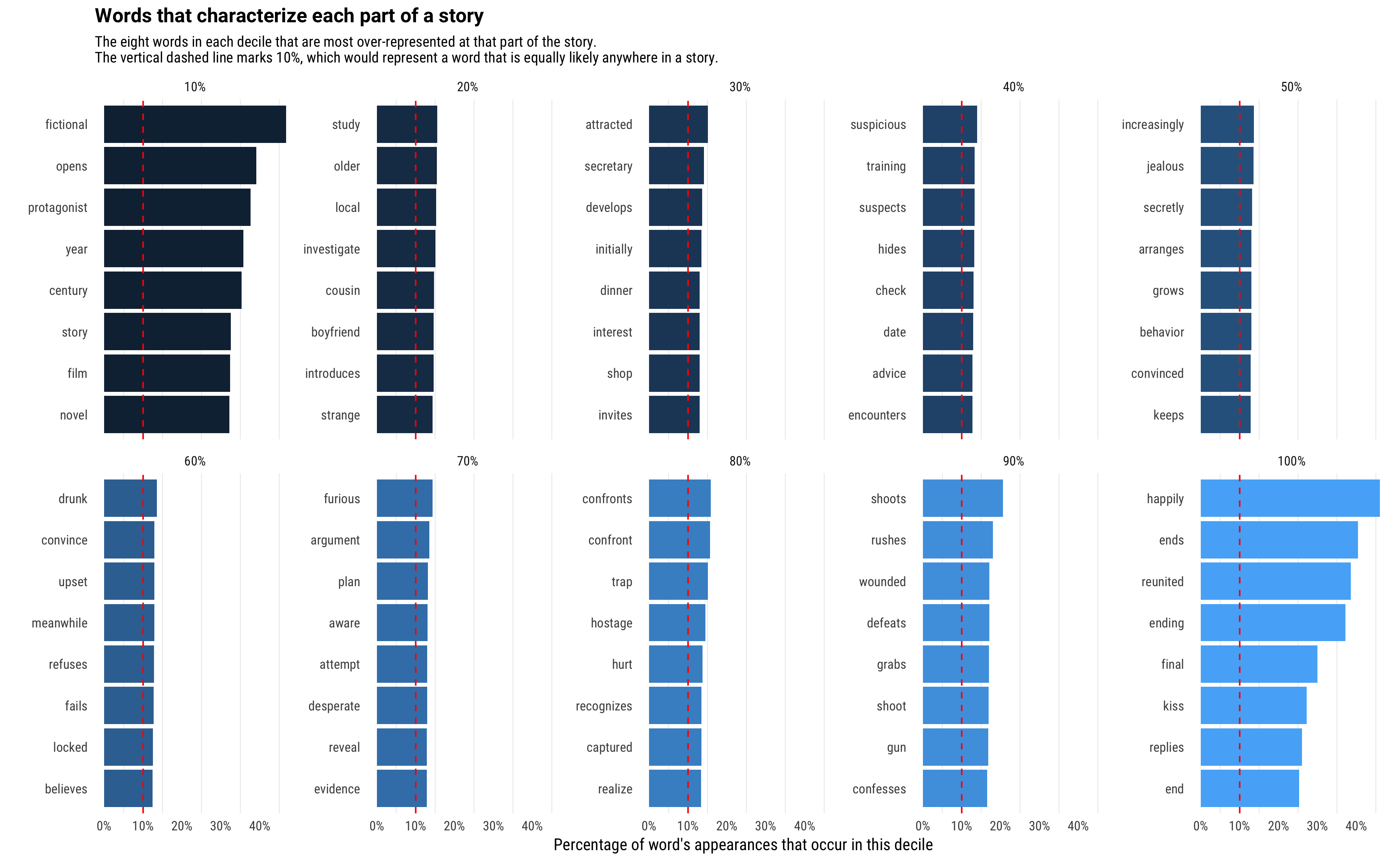
We see that the words in the start and the end are the most specific to their particular deciles: for example, almost half of the occurrences of the word “fictional” occurred in the first 10% of the story. The middle sections have words that are more spread out (having, say, 14% of their occurrences in that section rather than the expected 10%), but they still are words that make sense in the story structure.
Let’s visualize the full trend for the words overrepreseted at each point.
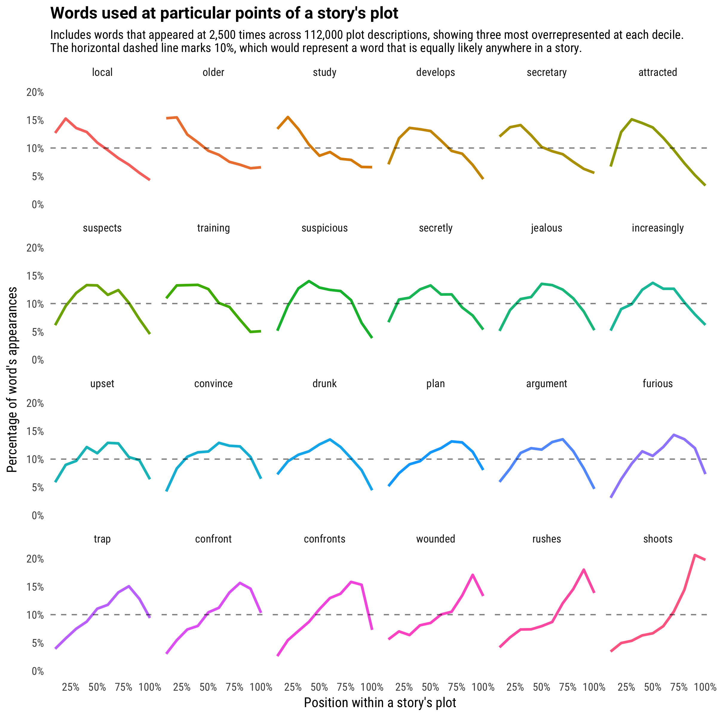
Try reading the 24 word story laid out by the subgraph titles. Our protagonist is “attracted”, then “suspicious”, followed by “jealous”, “drunk”, and ultimately “furious”. A shame that once they “confront” the problem, they run into a “trap” and are “wounded”. If you ignore the repetitive words and the lack of syntax, you can see the rising tension of a story just in these sparklines.
Sentiment analysis
As one more confirmation of our hypothesis about rising tension and conflict within a story, we can use sentiment analysis to find the average sentiment within each piece of a story.
decile_counts %>%
  inner_join(get_sentiments("afinn"), by = "word") %>%
  group_by(decile) %>%
  summarize(score = sum(score * n) / sum(n)) %>%
  ggplot(aes(decile, score)) +
  geom_line() +
  scale_x_continuous(labels = percent_format()) +
  expand_limits(y = 0) +
  labs(x = "Position within a story",
       y = "Average AFINN sentiment score")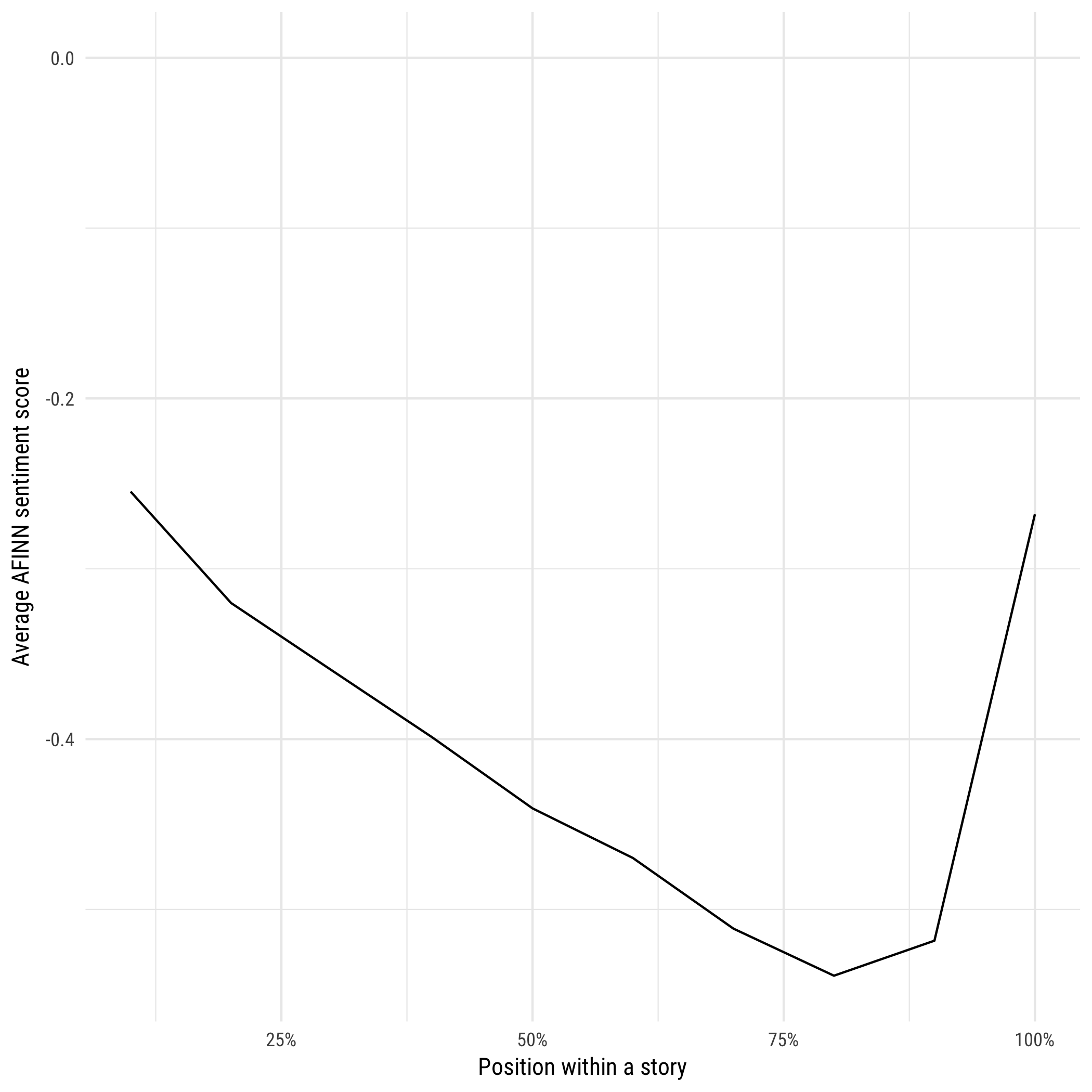
Plot descriptions have a negative average AFINN score at all points in the story (which makes sense, since stories focus on conflict. But it might start with a relatively peaceful beginning, before the conflict increases over the course of the plot, until it hits a maximum around the climax, 80-90%. It’s then often followed by a resolution, which contains words like “happily”, “rescues”, and “reunited” that return it to a higher sentiment score.
In short, if we had to summarize the average story that humans tell, it would go something like Things get worse and worse until at the last minute they get better.
To be continued
This was a pretty simple analysis of story arcs (for a more in-depth example, see the research described here), and it doesn’t tell us too much we wouldn’t have been able to guess. (Except perhaps that characters are most likely to be drunk right in the middle of a story. How can we monetize that insight?)
What I like about this approach is how quickly you can gain insights with simple quantitative methods (counting, taking the median) applied to a large text dataset. In future posts, I’ll be diving deeper into these plots and showing what else we can learn.