broom: a package for tidying statistical models into data frames

The concept of “tidy data”, as introduced by Hadley Wickham, offers a powerful framework for data manipulation, analysis, and visualization. Popular packages like dplyr, tidyr and ggplot2 take great advantage of this framework, as explored in several recent posts by others.

But there’s an important step in a tidy data workflow that so far has been missing: the output of R statistical modeling functions isn’t tidy, meaning it’s difficult to manipulate and recombine in downstream analyses and visualizations. Hadley’s paper makes a convincing statement of this problem (emphasis mine):

While model inputs usually require tidy inputs, such attention to detail doesn’t carry over to model outputs. Outputs such as predictions and estimated coefficients aren’t always tidy. This makes it more difficult to combine results from multiple models. For example, in R, the default representation of model coefficients is not tidy because it does not have an explicit variable that records the variable name for each estimate, they are instead recorded as row names. In R, row names must be unique, so combining coefficients from many models (e.g., from bootstrap resamples, or subgroups) requires workarounds to avoid losing important information. This knocks you out of the flow of analysis and makes it harder to combine the results from multiple models. I’m not currently aware of any packages that resolve this problem.

In this new paper I introduce the broom package (available on CRAN), which bridges the gap from untidy outputs of predictions and estimations to the tidy data we want to work with. It takes the messy output of built-in statistical functions in R, such as lm, nls, kmeans, or t.test, as well as popular third-party packages, like gam, glmnet, survival or lme4, and turns them into tidy data frames. This allows the results to be handed to other tidy packages for downstream analysis: they can be recombined using dplyr or visualized using ggplot2.

Example: linear regression

As a simple example, consider a linear regression on the built-in mtcars dataset:

fit <- lm(mpg ~ wt + qsec, mtcars)
summary(fit)

## 
## Call:
## lm(formula = mpg ~ wt + qsec, data = mtcars)
## 
## Residuals:
##     Min      1Q  Median      3Q     Max 
## -4.3962 -2.1431 -0.2129  1.4915  5.7486 
## 
## Coefficients:
##             Estimate Std. Error t value Pr(>|t|)    
## (Intercept)  19.7462     5.2521   3.760 0.000765 ***
## wt           -5.0480     0.4840 -10.430 2.52e-11 ***
## qsec          0.9292     0.2650   3.506 0.001500 ** 
## ---
## Signif. codes:  0 '***' 0.001 '**' 0.01 '*' 0.05 '.' 0.1 ' ' 1
## 
## Residual standard error: 2.596 on 29 degrees of freedom
## Multiple R-squared:  0.8264,	Adjusted R-squared:  0.8144 
## F-statistic: 69.03 on 2 and 29 DF,  p-value: 9.395e-12

This summary shows many kinds of statistics describing the regression: coefficient estimates and p-values, information about the residuals, and model statistics like $R^2$ and the F statistic. But this format isn’t convenient if you want to combine and compare multiple models, or plot it using ggplot2: you need to turn it into a data frame.

The broom package provides three tidying methods for turning the contents of this object into a data frame, depending on the level of statistics you’re interested in. If you want statistics about each of the coefficients fit by the model, use the tidy() method:

library(broom)
tidy(fit)

##          term  estimate std.error  statistic      p.value
## 1 (Intercept) 19.746223 5.2520617   3.759709 7.650466e-04
## 2          wt -5.047982 0.4839974 -10.429771 2.518948e-11
## 3        qsec  0.929198 0.2650173   3.506179 1.499883e-03

Note that the rownames are now added as a column, term, meaning that the data can be combined with other models. Note also that the columns have been given names like std.error and p.value that are more easily accessed than Std. Error and Pr(>|t|). This is true of all data frames broom returns: they’re designed so they can be processed in additional steps.

If you’re interested in extracting per-observation information, such as fitted values and residuals, use the augment() method, which adds these to the original data:

head(augment(fit))

##           .rownames  mpg    wt  qsec  .fitted   .se.fit      .resid
## 1         Mazda RX4 21.0 2.620 16.46 21.81511 0.6832424 -0.81510855
## 2     Mazda RX4 Wag 21.0 2.875 17.02 21.04822 0.5468271 -0.04822401
## 3        Datsun 710 22.8 2.320 18.61 25.32728 0.6397681 -2.52727880
## 4    Hornet 4 Drive 21.4 3.215 19.44 21.58057 0.6231436 -0.18056924
## 5 Hornet Sportabout 18.7 3.440 17.02 18.19611 0.5120709  0.50388581
## 6           Valiant 18.1 3.460 20.22 21.06859 0.8032106 -2.96858808
##         .hat   .sigma      .cooksd  .std.resid
## 1 0.06925986 2.637300 2.627038e-03 -0.32543724
## 2 0.04436414 2.642112 5.587076e-06 -0.01900129
## 3 0.06072636 2.595763 2.174253e-02 -1.00443793
## 4 0.05761138 2.641895 1.046036e-04 -0.07164647
## 5 0.03890382 2.640343 5.288512e-04  0.19797699
## 6 0.09571739 2.575422 5.101445e-02 -1.20244126

Finally, glance() computes per-model statistics, such as $R^2$, AIC, and BIC:

glance(fit)

##   r.squared adj.r.squared    sigma statistic      p.value df    logLik
## 1 0.8264161     0.8144448 2.596175  69.03311 9.394765e-12  3 -74.36025
##        AIC      BIC deviance df.residual
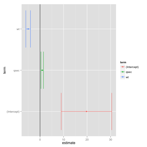
## 1 156.7205 162.5834 195.4636          29

As pointed out by Mike Love, the tidy method makes it easy to construct coefficient plots using ggplot2:

library(ggplot2)
td <- tidy(fit, conf.int = TRUE)
ggplot(td, aes(estimate, term, color = term)) +
    geom_point() +
    geom_errorbarh(aes(xmin = conf.low, xmax = conf.high)) +
    geom_vline()

When combined with dplyr’s group_by and do, broom also lets you perform regressions within groups, such as within automatic and manual cars separately:

library(dplyr)
mtcars %>% group_by(am) %>% do(tidy(lm(mpg ~ wt, .)))

## Source: local data frame [4 x 6]
## Groups: am
## 
##   am        term  estimate std.error statistic      p.value
## 1  0 (Intercept) 31.416055 2.9467213 10.661360 6.007748e-09
## 2  0          wt -3.785908 0.7665567 -4.938848 1.245595e-04
## 3  1 (Intercept) 46.294478 3.1198212 14.838824 1.276849e-08
## 4  1          wt -9.084268 1.2565727 -7.229401 1.687904e-05

This is useful for performing regressions or other analyses within each gene, country, or any other kind of division in your tidy dataset.

Using tidiers for visualization with ggplot2

The broom package provides tidying methods for many other packages as well. These tidiers serve to connect various statistical models seamlessly with packages like dplyr and ggplot2. For instance, we could create a LASSO regression with the glmnet package:

library(glmnet)
set.seed(03-19-2015)

# generate data with 5 real variables and 45 null, on 100 observations
nobs <- 100
nvar <- 50
real <- 5
x <- matrix(rnorm(nobs * nvar), nobs)
beta <- c(rnorm(real, 0, 1), rep(0, nvar - real))
y <- c(t(beta) %*% t(x)) + rnorm(nvar, sd = 3)

glmnet_fit <- cv.glmnet(x,y)

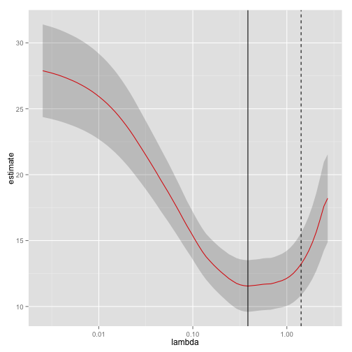
Then we tidy it with broom and plot it using ggplot2:

tidied_cv <- tidy(glmnet_fit)
glance_cv <- glance(glmnet_fit)

ggplot(tidied_cv, aes(lambda, estimate)) + geom_line(color = "red") +
    geom_ribbon(aes(ymin = conf.low, ymax = conf.high), alpha = .2) +
    scale_x_log10() +
    geom_vline(xintercept = glance_cv$lambda.min) +
    geom_vline(xintercept = glance_cv$lambda.1se, lty = 2)

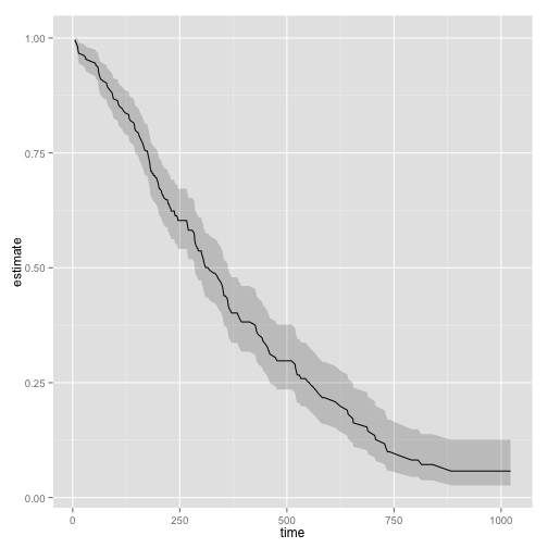
By plotting with ggplot2 rather than relying on glmnet’s built-in plotting methods, we gain access to all the tools and framework of the package. This allows us to customize or add attributes, or even to compare multiple LASSO cross-validations in the same plot. The same is true of the survival package:

library(survival)

surv_fit <- survfit(coxph(Surv(time, status) ~ age + sex, lung))

td <- tidy(surv_fit)
ggplot(td, aes(time, estimate)) + geom_line() +
    geom_ribbon(aes(ymin = conf.low, ymax = conf.high), alpha = .2)

Others have explored how broom can help visualize random effects estimated with lme4. Other packages for which tidiers are implemented include gam, zoo, lfe, and multcomp.

The vignettes for the broom package offer other useful examples, including one on combining broom and dplyr, a demonstration of bootstrapping with broom, and a simulation of k-means clustering. The broom manuscript offers still more examples.

Tidying model outputs is not an exact science, and it is based on a judgment of the kinds of values a data scientist typically wants out of a tidy analysis (for instance, estimates, test statistics, and p-values). It is my hope that data scientists will propose and contribute their own features feature requests are welcome!) to help expand the universe of tidy analysis tools.