
Yesterday a family member forwarded me a Wall Street Journal interview titled What Data Scientists Do All Day At Work. The title intrigued me immediately, partly because I find myself explaining that same topic somewhat regularly.
I wasn’t disappointed in the interview: General Electric’s Dr. Narasimhan gave insightful and well-communicated answers, and I both recognized familiar opinions and learned new perspectives. But I was disappointed that in an article about data scientists (!) they would include a chart this terrible:
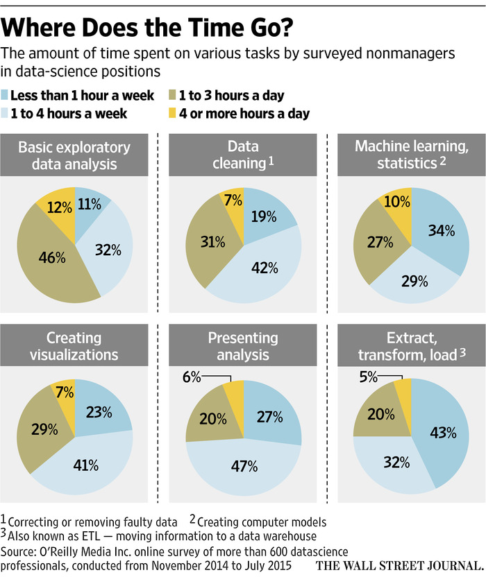
Pie charts have a bad reputation among statisticians and data scientists, with good reason (see here for more). But this is an especially unfortunate example. We’re meant to compare and contrast these six tasks. But at a glance, do you have any idea whether more time is spent “Presenting Analysis” or “Data cleaning”?
The problem with a lot of pie-chart bashing (and most “chart-shaming,” in fact) is that people don’t follow up with a better alternative. So here I’ll show how I would have created a different graph (using R and ggplot2) to communicate the same information. This also serves as an example of the thought process I go through in creating a data visualization.
(I’d note that this post is appropriate for Pi Day, but I’m more of a Tau Day observer anyway).
Setup
I start by transcribing the data directly from the plot into R. readr::read_csv is useful for constructing a table on the fly:
library(readr)

d <- read_csv("Task,< 1 a week,1-4 a week,1-3 a day,>4 a day
Basic exploratory data analysis,11,32,46,12
Data cleaning,19,42,31,7
Machine learning/statistics,34,29,27,10
Creating visualizations,23,41,29,7
Presenting analysis,27,47,20,6
Extract/transform/load,43,32,20,5")

# reorganize
library(tidyr)
d <- gather(d, Hours, Percentage, -Task)
This constructs our data in the form:1
| Task | Hours | Percentage |
|---|---|---|
| Basic exploratory data analysis | < 1 a week | 11 |
| Data cleaning | < 1 a week | 19 |
| Machine learning/statistics | < 1 a week | 34 |
| Creating visualizations | < 1 a week | 23 |
| Presenting analysis | < 1 a week | 27 |
| Extract/transform/load | < 1 a week | 43 |
| Basic exploratory data analysis | 1-4 a week | 32 |
| Data cleaning | 1-4 a week | 42 |
| Machine learning/statistics | 1-4 a week | 29 |
Bar plot
The most common way a pie chart can be improved is by turning it into a bar chart, with categories on the x axis and percentages on the y-axis.
This doesn’t apply to all plots, but it does to this one.
library(ggplot2)
theme_set(theme_bw())

ggplot(d, aes(Hours, Percentage)) +
  geom_bar(stat = "identity") +
  facet_wrap(~Task)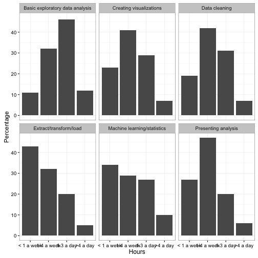
Note that much like the original pie chart, we “faceted” (divided into sub-plots) based on the Task.
This graph is not yet polished, but notice that it’s already easier to tell how the distribution of responses differs between tasks. This is because the x-axis is ordered from left to right as “spend a little time” to “spend a lot of time”- therefore, the more “right shifted” each graph is, the more time is spent on it. Notice also that we were able to drop the legend, which makes the plot both take up less space and require less looking back and forth.
Alternative plots
This was one of a few alternatives I considered when I first imagined creating the plot. When you’ve made a lot of plots, you’ll learn to guess in advance which you will be worth trying, but often it’s worth visualizing a few just to check.
We have three attributes in our data: Hours, Task, and Percentage. We chose to use x, y, and facet to communicate those respectively, but we could have chosen other arrangements. For example, we could have had Task represented by color, and represented it with a line plot:
ggplot(d, aes(Hours, Percentage, color = Task, group = Task)) +
  geom_line()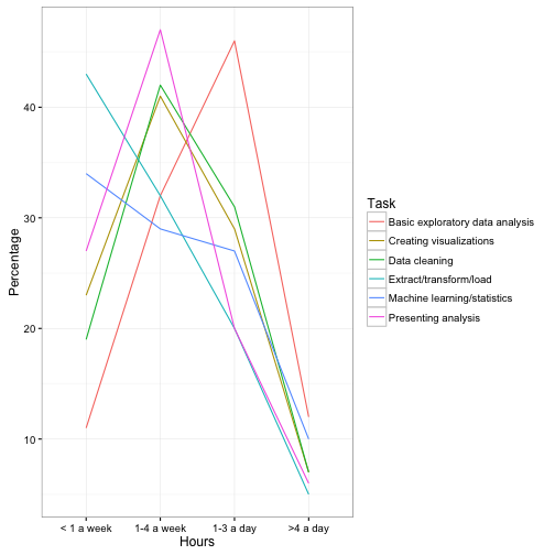
This has some advantages over the above bar chart. For starters, it makes it trivially easy to compare two tasks. (For example, we learn that “Creating visualizations” and “Data cleaning” take about the same distribution of time). I also like how obvious it makes it that “Basic exploratory data analysis” takes up more time than the others. But the graph makes it harder to focus just one one task, you have to look back and forth from the legend, and there’s almost no way we could annotate it with text like the original plot was.
Here’s another combination we could try:
ggplot(d, aes(Hours, Task, fill = Percentage)) +
  geom_tile(show.legend = FALSE) +
  geom_text(aes(label = paste0(Percentage, "%")), color = "white")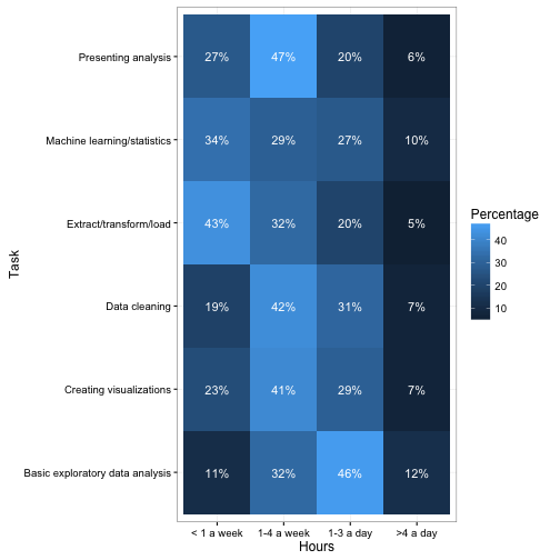
This approach is more of a “table”. This communicates a bit less than the bar and line plots since it gives up the y/size aesthetic for communicating Percentage. But notice that it’s still about as easy to interpret as the pie chart, simply because it is able to communicate the “left-to-right” ordering of “less time to more time”.
Improving our graph
How can our bar plot be improved?
The first problem that jumps out is that the x-axis overlaps so the labels are nearly unreadable. This can be fixed with this solution.
ggplot(d, aes(Hours, Percentage)) +
  geom_bar(stat = "identity") +
  facet_wrap(~Task) +
  theme(axis.text.x = element_text(angle = 90,  hjust = 1))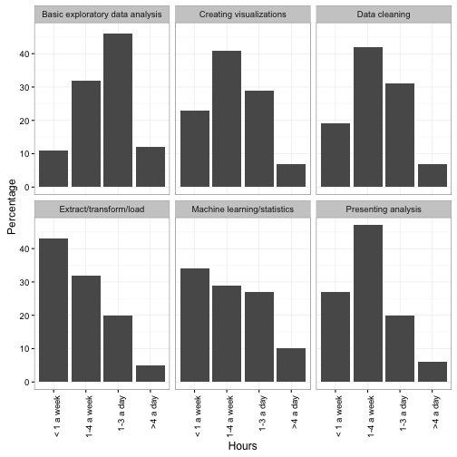
Next, note that the original pie chart showed the percentages as text right on the graph. This was necessary in the pie chart simply because it’s so difficult to guess a percentage out of a pie chart- we could afford to lose it here, when the y-axis communicates the same information. But it can still be useful when you want to pick out a specific number to report (“Visualization is important: 7% of data scientists spend >4 hours a day on it!”) So I add a geom_text layer.
ggplot(d, aes(Hours, Percentage)) +
  geom_bar(stat = "identity") +
  facet_wrap(~Task) +
  geom_text(aes(label = paste0(Percentage, "%"), y = Percentage),
            vjust = 1.4, size = 5, color = "white")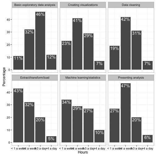
The ordering of task facets is arbitrary (alphabetical in this plot). I like to give them an order that makes them easier to browse- something along the lines of. A simple proxy for this is to order by “% who spend < 1 hour a week.”2
library(dplyr)

d %>%
  mutate(Task = reorder(Task, Percentage, function(e) e[1])) %>%
  ggplot(aes(Hours, Percentage)) +
  geom_bar(stat = "identity") +
  facet_wrap(~Task) +
  geom_text(aes(label = paste0(Percentage, "%"), y = Percentage),
            vjust = 1.4, size = 5, color = "white") +
  theme(axis.text.x = element_text(angle = 90,  hjust = 1)) +
  xlab("Hours spent per week")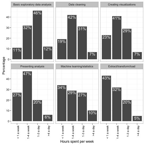
Graph design
From here, the last step would be to adjust the colors, fonts, and other “design” choices.
I don’t have terribly strong opinions about these choices (I’m pretty happy with ggplot2’s theme_bw()). But some prefer Edward Tufte’s approach of maximizing the “Data/Ink Ratio”- that is, dropping borders, grids, and axis lines. This can be achieved with theme_tufte:
library(ggthemes)

d %>%
  mutate(Task = reorder(Task, Percentage, function(e) e[1])) %>%
  ggplot(aes(Hours, Percentage)) +
  geom_bar(stat = "identity") +
  facet_wrap(~Task) +
  geom_text(aes(label = paste0(Percentage, "%"), y = Percentage),
            vjust = 1.4, size = 5, color = "white") +
  theme_tufte() +
  theme(axis.text.x = element_text(angle = 90,  hjust = 1))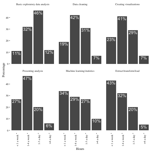
Some people take this philosophy even further, and drop the y-axis altogether (since we do already have those percentages annotated on the bars).
library(ggthemes)

d %>%
  mutate(Task = reorder(Task, Percentage, function(e) e[1])) %>%
  ggplot(aes(Hours, Percentage)) +
  geom_bar(stat = "identity") +
  facet_wrap(~Task) +
  geom_text(aes(label = paste0(Percentage, "%"), y = Percentage),
            vjust = 1.4, size = 5, color = "white") +
  theme_tufte() +
  theme(axis.text.x = element_text(angle = 90,  hjust = 1),
        axis.ticks = element_blank(),
        axis.text.y = element_blank()) +
  ylab("")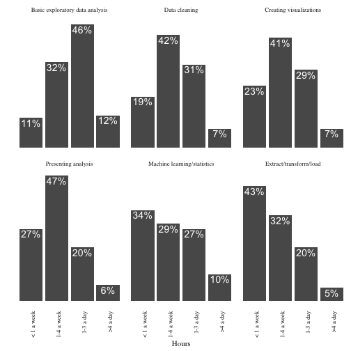
(See here for an animated version of this “Less is more” philosophy).
So take a look at the two versions:
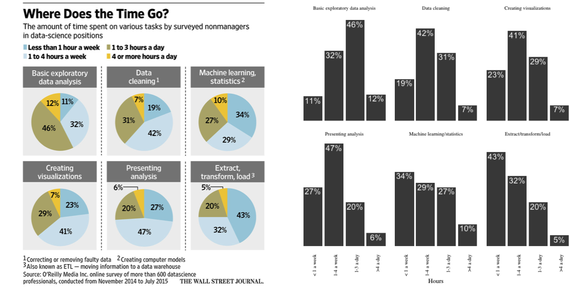
Which communicates more to you? And can you think of a plot that communicates this data even more clearly?
Postscript: How would I do this in base R plotting?
Footnotes
-
Why did I choose to represent it in this “gathered” format, rather than one row per task and one column per hour? Because using tidy data makes it easier to plot! ↩
-
This isn’t actually going to tell us which tasks data scientists spend the most time on: we should do some kind of weighted measure to estimate the mean. But for visualization purposes this is enough. ↩