
At Stack Overflow we’ve always been committed to sharing data: all content contributed to the site is CC-BY-SA licensed, and we release regular “data dumps” of our entire history of questions and answers.
I’m excited to announce a new resource specially aimed at data scientists, analysts and other researchers, which we’re calling the StackLite dataset.
What’s in the StackLite dataset?
For each Stack Overflow question asked since the beginning of the site, the dataset includes:
- Question ID
- Creation date
- Closed date, if applicable
- Deletion date, if applicable
- Score
- Owner user ID (except for deleted questions)
- Number of answers
- Tags
This is ideal for performing analyses such as:
- The increase or decrease in questions in each tag over time
- Correlations among tags on questions
- Which tags tend to get higher or lower scores
- Which tags tend to be asked on weekends vs weekdays
- Rates of question closure or deletion over time
- The speed at which questions are closed or deleted
Examples in R
The dataset is provided as csv.gz files, which means you can use almost any language or statistical tool to process it. But here I’ll share some examples of a simple analysis in R.
The question data and the question-tag pairings are stored separately. You can read in the dataset (once you’ve cloned or downloaded it from GitHub) with:
library(readr)
library(dplyr)

questions <- read_csv("stacklite/questions.csv.gz")
question_tags <- read_csv("stacklite/question_tags.csv.gz")
The questions file has one row for each question:
questions## Source: local data frame [15,497,156 x 7]
##
## Id CreationDate ClosedDate DeletionDate Score
## (int) (time) (time) (time) (int)
## 1 1 2008-07-31 21:26:37 <NA> 2011-03-28 00:53:47 1
## 2 4 2008-07-31 21:42:52 <NA> <NA> 406
## 3 6 2008-07-31 22:08:08 <NA> <NA> 181
## 4 8 2008-07-31 23:33:19 2013-06-03 04:00:25 2015-02-11 08:26:40 42
## 5 9 2008-07-31 23:40:59 <NA> <NA> 1286
## 6 11 2008-07-31 23:55:37 <NA> <NA> 1046
## 7 13 2008-08-01 00:42:38 <NA> <NA> 415
## 8 14 2008-08-01 00:59:11 <NA> <NA> 265
## 9 16 2008-08-01 04:59:33 <NA> <NA> 65
## 10 17 2008-08-01 05:09:55 <NA> <NA> 96
## .. ... ... ... ... ...
## Variables not shown: OwnerUserId (int), AnswerCount (int)While the question_tags file has one row for each question-tag pair:
question_tags## Source: local data frame [45,510,638 x 2]
##
## Id Tag
## (int) (chr)
## 1 1 data
## 2 4 c#
## 3 4 winforms
## 4 4 type-conversion
## 5 4 decimal
## 6 4 opacity
## 7 6 html
## 8 6 css
## 9 6 css3
## 10 6 internet-explorer-7
## .. ... ...As one example, you could find the most popular tags:
question_tags %>%
  count(Tag, sort = TRUE)
## Source: local data frame [55,661 x 2]
##
## Tag n
## (chr) (int)
## 1 javascript 1454248
## 2 java 1409336
## 3 php 1241691
## 4 c# 1208953
## 5 android 1163810
## 6 jquery 931882
## 7 python 732188
## 8 html 690762
## 9 ios 573246
## 10 c++ 571386
## .. ... ...Or plot the number of questions asked per week:
library(ggplot2)
library(lubridate)

questions %>%
  count(Week = round_date(CreationDate, "week")) %>%
  ggplot(aes(Week, n)) +
  geom_line()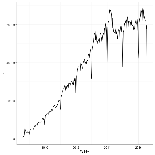
Many of the most interesting issues you can examine involve tags, which describe the programming language or technology used in a question. You could compare the growth or decline of particular tags over time:
library(lubridate)

tags <- c("c#", "javascript", "python", "r")

q_per_year <- questions %>%
  count(Year = year(CreationDate)) %>%
  rename(YearTotal = n)

tags_per_year <- question_tags %>%
  filter(Tag %in% tags) %>%
  inner_join(questions) %>%
  count(Year = year(CreationDate), Tag) %>%
  inner_join(q_per_year)

ggplot(tags_per_year, aes(Year, n / YearTotal, color = Tag)) +
  geom_line() +
  scale_y_continuous(labels = scales::percent_format()) +
  ylab("% of Stack Overflow questions with this tag")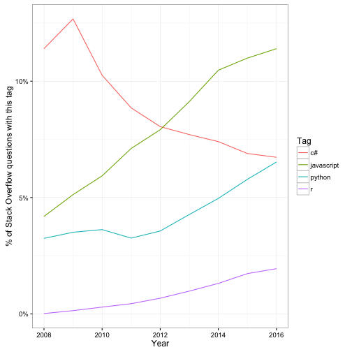
How this compares to other Stack Overflow resources
Almost all of this data is already public within the Stack Exchange Data Dump. But the official data dump requires a lot of computational overhead to download and process (the Posts fit in a 27 GB XML file), even if the question you want to ask is very simple. The StackLite dataset, in contrast, is designed to be easy to read in and start analyzing. (For example, I was really impressed with Joshua Kunst’s analysis of tags over time, and want to make it straightforward for others to write posts like that).
Similarly, this data can be examined within the Stack Exchange Data Explorer (SEDE), but it requires working with separate queries that each return at most 50,000 rows. The StackLite dataset offers analysts the chance to work with the data locally using their tool of choice.
Enjoy!
I’m hoping other analysts find this dataset interesting, and use it to perform meaningful and open research. (Be sure to comment below if you do!)
I’m especially happy to have this dataset public and easily accessible, since it gives me the chance to blog more analyses of Stack Overflow questions and tags while keeping my work reproducible and extendable by others. Keep an eye out for such posts in the future!