
Previously in this series
- Understanding the beta distribution (using baseball statistics)
- Understanding empirical Bayes estimation (using baseball statistics)
- Understanding credible intervals (using baseball statistics)
- Understanding the Bayesian approach to false discovery rates (using baseball statistics)
Who is a better batter: Mike Piazza or Hank Aaron?
Well, Mike Piazza has a slightly higher career batting average (2127 hits / 6911 at-bats = 0.308) than Hank Aaron (3771 hits / 12364 at-bats = 0.305). But can we say with confidence that his skill is actually higher, or is it possible he just got lucky a bit more often?
In this series of posts about an empirical Bayesian approach to batting statistics, we’ve been estimating batting averages by modeling them as a binomial distribution with a beta prior. But we’ve been looking at a single batter at a time. What if we want to compare two batters, give a probability that one is better than the other, and estimate by how much?
This is a topic rather relevant to my own work and to the data science field, because understanding the difference between two proportions is important in A/B testing. One of the most common examples of A/B testing is comparing clickthrough rates (“out of X impressions, there have been Y clicks”)- which on the surface is similar to our batting average estimation problem (“out of X at-bats, there have been Y hits””).1
Here, we’re going to look at an empirical Bayesian approach to comparing two batters.2 We’ll define the problem in terms of the difference between each batter’s posterior distribution, and look at four mathematical and computational strategies we can use to resolve this question. While we’re focusing on baseball here, remember that similar strategies apply to A/B testing, and indeed to many Bayesian models.
Setup
I’ll start with some code you can use to catch up if you want to follow along in R. If you want to understand what the code does, check out the previous posts. (All the code in this post, including for the figures where code isn’t shown, can be found here).
library(dplyr)
library(tidyr)
library(Lahman)

# Grab career batting average of non-pitchers
# (allow players that have pitched <= 3 games, like Ty Cobb)
pitchers <- Pitching %>%
  group_by(playerID) %>%
  summarize(gamesPitched = sum(G)) %>%
  filter(gamesPitched > 3)

career <- Batting %>%
  filter(AB > 0) %>%
  anti_join(pitchers, by = "playerID") %>%
  group_by(playerID) %>%
  summarize(H = sum(H), AB = sum(AB)) %>%
  mutate(average = H / AB)

# Add player names
career <- Master %>%
  tbl_df() %>%
  select(playerID, nameFirst, nameLast) %>%
  unite(name, nameFirst, nameLast, sep = " ") %>%
  inner_join(career, by = "playerID")

# Estimate hyperparameters alpha0 and beta0 for empirical Bayes
career_filtered <- career %>% filter(AB >= 500)
m <- MASS::fitdistr(career_filtered$average, dbeta,
                    start = list(shape1 = 1, shape2 = 10))

alpha0 <- m$estimate[1]
beta0 <- m$estimate[2]

# For each player, update the beta prior based on the evidence
# to get posterior parameters alpha1 and beta1
career_eb <- career %>%
  mutate(eb_estimate = (H + alpha0) / (AB + alpha0 + beta0)) %>%
  mutate(alpha1 = H + alpha0,
         beta1 = AB - H + beta0) %>%
  arrange(desc(eb_estimate))
So let’s take a look at the two batters in question:
# while we're at it, save them as separate objects too for later:
aaron <- career_eb %>% filter(name == "Hank Aaron")
piazza <- career_eb %>% filter(name == "Mike Piazza")
two_players <- bind_rows(aaron, piazza)

two_players
## Source: local data frame [2 x 8]
##
## playerID name H AB average eb_estimate alpha1 beta1
## (chr) (chr) (int) (int) (dbl) (dbl) (dbl) (dbl)
## 1 aaronha01 Hank Aaron 3771 12364 0.305 0.304 3847 8812
## 2 piazzmi01 Mike Piazza 2127 6911 0.308 0.306 2203 5003We see that Piazza has a slightly higher average (\(H / AB\)), and a higher shrunken empirical bayes estimate (\((H + \alpha_0) / (AB + \alpha_0 + \beta_0)\), where \(\alpha_0\) and \(\beta_0\) are our priors).
But is Piazza’s true probability of getting a hit higher? Or is the difference due to chance? To answer, let’s consider the actual posterior distributions- the range of plausible values for their “true” batting averages after we’ve taken the evidence (their batting record) into account. Recall that these posterior distributions are modeled as beta distributions with the parameters \(\mbox{Beta}(\alpha_0 + H, \alpha_0 + \beta_0 + H + AB)\).
library(broom)
library(ggplot2)
theme_set(theme_bw())

two_players %>%
  inflate(x = seq(.28, .33, .00025)) %>%
  mutate(density = dbeta(x, alpha1, beta1)) %>%
  ggplot(aes(x, density, color = name)) +
  geom_line() +
  labs(x = "Batting average", color = "")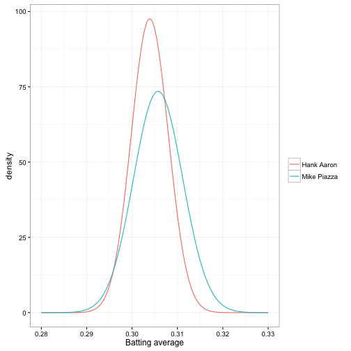
This posterior is a probabilistic representation of our uncertainty in each estimate. Thus, when asking the probability Piazza is better, we’re asking “if I drew a random draw from Piazza’s and a random draw from Aaron’s, what’s the probability Piazza is higher”?
Well, notice that those two distributions overlap a lot! There’s enough uncertainty in each of those estimates that Aaron could easily be better than Piazza.
Let’s throw another player in, retired Yankee Hideki Matsui:
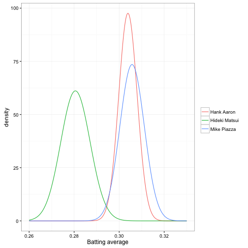
Hideki Matsui is a fine batter (above average for major league baseball), but not up to the level of Aaron and Piazza: notice that his posterior distribution barely overlaps theirs. If we took a random draw from Matsui’s distribution and from Piazza’s, it’s very unlikely Matsui’s would be higher.
Posterior Probability
We may be interested in the probability that Piazza is better than Aaron within our model. We can already tell from the graph that it’s greater than 50%, but probably not much greater. How could we quantify it?
We’d need to know the probability one beta distribution is greater than another. This question is not trivial to answer, and I’m going to illustrate four routes that are common lines of attack in a Bayesian problem:
- Simulation of posterior draws
- Numerical integration
- Closed-form solution
- Closed-form approximation
Which of these approaches you choose depends on your particular problem, as well as your computational constraints. In many cases an exact closed-form solution may not be known or even exist. In some cases (such as running machine learning in production) you may be heavily constrained for time, while in others (such as drawing conclusions for a scientific paper) you care more about precision.
Simulation of posterior draws
If we don’t want to do any math today (I hear you), we could simply try simulation. We could use each player’s \(\alpha_1\) and \(\beta_1\) parameters, draw a million items from each of them using rbeta, and compare the results:
piazza_simulation <- rbeta(1e6, piazza$alpha1, piazza$beta1)
aaron_simulation <- rbeta(1e6, aaron$alpha1, aaron$beta1)

sim <- mean(piazza_simulation > aaron_simulation)
sim
## [1] 0.607So about 60.7% probability Piazza is better than Aaron! An answer like this is often good enough, depending on your need for precision and the computational efficiency. You could turn up or down the number of draws depending on how much you value speed vs precision.
Notice we didn’t have to do any mathematical derivation or proofs. Even if we had a much more complicated model, the process for simulating from it would still have been pretty straightforward. This is one of the reasons Bayesian simulation approaches like MCMC have become popular: computational power has gotten very cheap, while doing math is as expensive as ever.
Integration
These two posteriors each have their own (independent) distribution, and together they form a joint distribution- that is, a density over particular pairs of \(x\) and \(y\). That joint distribution could be imagined as a density cloud:
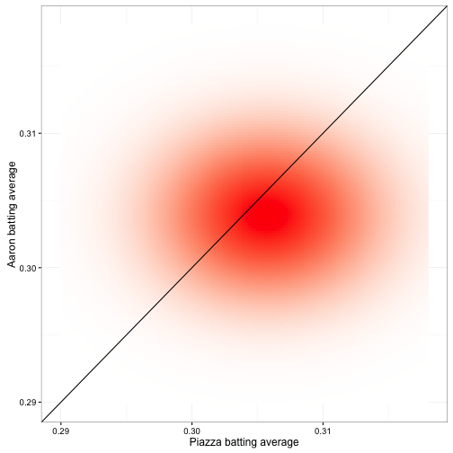
Here, we’re asking what fraction of the joint probability density lies below that black line, where Piazza’s average is greater than Aaron’s. Notice that more of it lies below than above: that’s confirming the posterior probability that Piazza is better is about 60%.
The way to calculate this quantitatively is numerical integration, which is how Chris Stucchio approaches the problem in this post and this Python script. A simple approach in R would be something like:
d <- .00002
limits <- seq(.29, .33, d)
sum(outer(limits, limits, function(x, y) {
  (x > y) *
    dbeta(x, piazza$alpha1, piazza$beta1) *
    dbeta(y, aaron$alpha1, aaron$beta1) *
    d ^ 2
}))
## [1] 0.606Like simulation, this is a bit on the “brute force” side. (And unlike simulation, the approach becomes intractable in problems that have many dimensions, as opposed to the two dimensions here).
Closed-form solution
You don’t need to be great at calculus to be a data scientist. But it’s useful to know how to find people that are great at calculus. When it comes to A/B testing, the person to find is often Evan Miller.
This post lays out a closed-form solution Miller derived for the probability a draw from one beta distribution is greater than a draw from another:
\[p_A \sim \mbox{Beta}(\alpha_A, \beta_A)\] \[p_B \sim \mbox{Beta}(\alpha_B, \beta_B)\] \[{\rm Pr}(p_B > p_A) = \sum_{i=0}^{\alpha_B-1}\frac{B(\alpha_A+i,\beta_A+\beta_B)}{(\beta_B+i) B(1+i, \beta_B) B(\alpha_A, \beta_A) }\](Where \(B\) is the beta function). If you’d like an intuition behind this formula… well, you’re on your own. But it’s pretty straightforward to implement in R (I’m borrowing notation from this post and calling it \(h\)):
h <- function(alpha_a, beta_a,
              alpha_b, beta_b) {
  j <- seq.int(0, round(alpha_b) - 1)
  log_vals <- (lbeta(alpha_a + j, beta_a + beta_b) - log(beta_b + j) -
               lbeta(1 + j, beta_b) - lbeta(alpha_a, beta_a))
  1 - sum(exp(log_vals))
}

h(piazza$alpha1, piazza$beta1,
  aaron$alpha1, aaron$beta1)
## [1] 0.608Having an exact solution is pretty handy!3 So why did we even look at simulation/integration approaches? Well, the downsides are:
- Not every problem has a solution like this. And even if it does, we may not know it. That’s why it’s worth knowing how to run a simulation. (If nothing else, they let us check our math!)
- This solution is slow for large \(\alpha_B\), and not straightforward to vectorize: notice that term that iterates from 0 to \(\alpha_B-1\). If we run A/B tests with thousands of clicks, this step is going to constrain us (though it’s still usually faster than simulation or integration).
Closed-form approximation
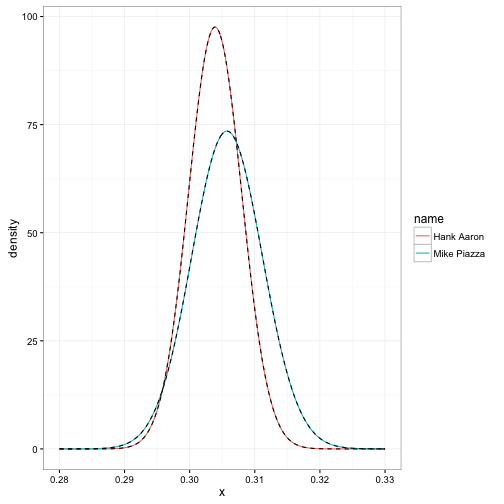
As this report points out, there’s a much faster approximation we can use. Notice that when \(\alpha\) and \(\beta\) are both fairly large, the beta starts looking a lot like a normal distribution, so much so that it can be closely approximated. In fact, if you draw the normal approximation to the two players we’ve been considering (shown as dashed line), they are visually indistinguishable:
And the probability one normal is greater than another is very easy to calculate- much easier than the beta!
h_approx <- function(alpha_a, beta_a,
                     alpha_b, beta_b) {
  u1 <- alpha_a / (alpha_a + beta_a)
  u2 <- alpha_b / (alpha_b + beta_b)
  var1 <- alpha_a * beta_a / ((alpha_a + beta_a) ^ 2 * (alpha_a + beta_a + 1))
  var2 <- alpha_b * beta_b / ((alpha_b + beta_b) ^ 2 * (alpha_b + beta_b + 1))
  pnorm(0, u2 - u1, sqrt(var1 + var2))
}

h_approx(piazza$alpha1, piazza$beta1, aaron$alpha1, aaron$beta1)
## [1] 0.607This calculation is very fast, and (in R terms) it’s vectorizable.
The disadvantage is that for low \(\alpha\) or low \(\beta\), the normal approximation to the beta is going to fit rather poorly. While the simulation and integration approaches were inexact, this one will be systematically biased: in some cases it will always give too high an answer, and in some cases too low. But when we have priors \(\alpha_0=76.451\) and \(\beta_0=218.639\), as we do here, our parameters are never going to be low, so we’re safe using it.
Confidence and credible intervals
In classical (frequentist) statistics, you may have seen this kind of “compare two proportions” problem before, perhaps laid out as a “contingency table”:
| Player | Hits | Misses |
|---|---|---|
| Hank Aaron | 3771 | 8593 |
| Mike Piazza | 2127 | 4784 |
One of the most common classical ways to approach these contingency table problems is with Pearson’s chi-squared test, implemented in R as prop.test:
prop.test(two_players$H, two_players$AB)##
## 2-sample test for equality of proportions with continuity
## correction
##
## data: two_players$H out of two_players$AB
## X-squared = 0.1, df = 1, p-value = 0.7
## alternative hypothesis: two.sided
## 95 percent confidence interval:
## -0.0165 0.0109
## sample estimates:
## prop 1 prop 2
## 0.305 0.308We see a non-significant p-value of .70. We won’t talk about p-values here (we talked a little about ways to translate between p-values and posterior probabilities in the last post). But we can agree it would have been strange if the p-value were significant, given that the posterior distributions overlapped so much.
Something else useful that prop.test gives you is a confidence interval for the difference between the two players. We learned in a previous post about credible intervals in terms of each player’s average. Now we’ll use empirical Bayes to compute the credible interval about the difference in these two players.
We could do this with simulation or integration, but let’s use our normal approximation approach (we’ll also compute our posterior probability while we’re at it):
credible_interval_approx <- function(a, b, c, d) {
  u1 <- a / (a + b)
  u2 <- c / (c + d)
  var1 <- a * b / ((a + b) ^ 2 * (a + b + 1))
  var2 <- c * d / ((c + d) ^ 2 * (c + d + 1))

  mu_diff <- u2 - u1
  sd_diff <- sqrt(var1 + var2)

  data_frame(posterior = pnorm(0, mu_diff, sd_diff),
             estimate = mu_diff,
             conf.low = qnorm(.025, mu_diff, sd_diff),
             conf.high = qnorm(.975, mu_diff, sd_diff))
}

credible_interval_approx(piazza$alpha1, piazza$beta1, aaron$alpha1, aaron$beta1)
## Source: local data frame [1 x 4]
##
## posterior estimate conf.low conf.high
## (dbl) (dbl) (dbl) (dbl)
## 1 0.607 -0.00185 -0.0152 0.0115It’s not particularly exciting for this Piazza/Aaron comparison (notice it’s very close to the confidence interval we calculated with prop.test). So let’s select 20 random players, and compare each of them to Mike Piazza. We’ll also calculate the confidence interval using prop.test, and compare them.
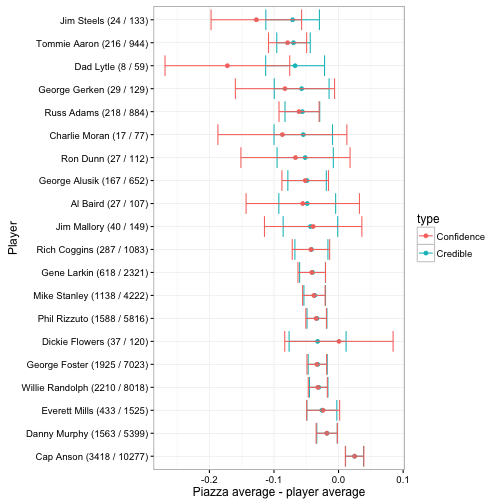
Notice the same pattern we saw in the credible intervals post. When we don’t have a lot of information about a player, their credible interval ends up smaller than their confidence interval, because we’re able to use the prior to adjust our expectations (Dad Lytle’s batting average may be lower than Mike Piazza’s, but we’re confident it’s not .25 lower). When we do have a lot of information, the credible intervals and confidence intervals converge almost perfectly.4
Thus, we can think of empirical Bayes A/B credible intervals as being a way to “shrink” frequentist confidence intervals, by sharing power across players.
Bayesian FDR control
Suppose we were a manager considering trading Piazza for another player (and suppose we could pick anyone from history). How many players in MLB history are we confident are better than Mike Piazza?
Well, we can compute the posterior probability and credible interval for each of them.
career_eb_vs_piazza <- bind_cols(
  career_eb,
  credible_interval_approx(piazza$alpha1, piazza$beta1,
                           career_eb$alpha1, career_eb$beta1)) %>%
  select(name, posterior, conf.low, conf.high)

career_eb_vs_piazza
## Source: local data frame [10,388 x 4]
##
## name posterior conf.low conf.high
## (chr) (dbl) (dbl) (dbl)
## 1 Ty Cobb 7.63e-17 0.0441 0.0716
## 2 Rogers Hornsby 2.81e-11 0.0345 0.0640
## 3 Shoeless Joe Jackson 8.42e-08 0.0279 0.0613
## 4 Ross Barnes 3.61e-05 0.0214 0.0633
## 5 Ed Delahanty 7.03e-07 0.0219 0.0518
## 6 Tris Speaker 1.57e-07 0.0225 0.0505
## 7 Ted Williams 1.45e-06 0.0206 0.0504
## 8 Billy Hamilton 6.91e-06 0.0190 0.0503
## 9 Levi Meyerle 4.01e-03 0.0087 0.0580
## 10 Harry Heilmann 7.15e-06 0.0180 0.0476
## .. ... ... ... ...While Piazza is an excellent batter, it looks like some do give him a run for his money. For instance, Ty Cobb has a batting average that’s about .04%-.07% better, with only a miniscule posterior probability that we’re wrong.
In order to get a set of players we’re confident are better (a set of candidates for trading), we can use the same approach to setting a false discovery rate (FDR) that we did in this post: taking the cumulative mean of the posterior error probability to compute the q-value.
career_eb_vs_piazza <- career_eb_vs_piazza %>%
  arrange(posterior) %>%
  mutate(qvalue = cummean(posterior))
Recall that the way we find a set of hypotheses with a given false discovery rate (FDR) is by filtering for a particular q-value:
better <- career_eb_vs_piazza %>%
  filter(qvalue < .05)

better
## Source: local data frame [65 x 5]
##
## name posterior conf.low conf.high qvalue
## (chr) (dbl) (dbl) (dbl) (dbl)
## 1 Ty Cobb 7.63e-17 0.0441 0.0716 7.63e-17
## 2 Rogers Hornsby 2.81e-11 0.0345 0.0640 1.41e-11
## 3 Shoeless Joe Jackson 8.42e-08 0.0279 0.0613 2.81e-08
## 4 Tris Speaker 1.57e-07 0.0225 0.0505 6.03e-08
## 5 Ed Delahanty 7.03e-07 0.0219 0.0518 1.89e-07
## 6 Ted Williams 1.45e-06 0.0206 0.0504 3.99e-07
## 7 Willie Keeler 4.62e-06 0.0183 0.0473 1.00e-06
## 8 Billy Hamilton 6.91e-06 0.0190 0.0503 1.74e-06
## 9 Harry Heilmann 7.15e-06 0.0180 0.0476 2.34e-06
## 10 Lou Gehrig 1.43e-05 0.0167 0.0461 3.54e-06
## .. ... ... ... ... ...This gives us 65 players we can say are better than Piazza, with an FDR of 5%. (That is, we expect we’re wrong on about 5% of this list of players).
What’s Next: Hierarchical modeling
We’re treating all baseball players as making up one homogeneous pool, whether they played in 1916 or 2016, and whether they played for the New York Yankees or the Chicago Cubs. This is mathematically convenient, but it’s ignoring a lot of information about players. One especially important piece of information it’s ignoring is how long someone played. Someone who’s been up to bat 5 or 6 times is generally not as good as someone with a 10-year career. This leads to a substantial bias where empirical Bayes tends to overestimate players with very few at-bats.
In the next post, we’ll talk about Bayesian hierarchical modeling, where rather than every player having the same prior, we allow the prior to depend on other known information. This will get us more accurate and reliable batting average estimates, while also extracting useful insights about factors that influence batters.
Further Reading
Above I’ve linked to a few great posts about Bayesian A/B testing, but here they are rounded up:
- Agile A/B testing with Bayesian Statistics and Python, by Chris Stucchio (the Bayesian Witch site appears to be down, so this links to an Internet Archive version)
- A Formula for Bayesian A/B Testing, by Evan Miller
- Easy Evaluation of Decision Rules in Bayesian A/B testing, by Chris Stucchio
Footnotes
-
The differences between frequentist and Bayesian A/B testing is a topic I’ve blogged about before, particularly about the problem of early stopping ↩
-
Don’t forget that I’m focusing on the elementary statistical concepts, not the baseball, in these posts. I’m not actually any good at sabermetrics- in a real analysis comparing players, you would control for many factors like the pitchers each faced and the stadiums they played in. ↩
-
Note that this solution is exact only for integer values of \(\alpha_b\): we’re rounding it here, which is a trivial difference in most of our examples but may matter in others. ↩
-
This can be derived mathematically, based on the fact that
prop.test’s confidence interval is in fact very similar to our normal approximation along with an uninformative prior and a small continuity correction, but it’s left as an exercise for the reader. ↩