
Previously in this series
- Understanding the beta distribution (using baseball statistics)
- Understanding empirical Bayes estimation (using baseball statistics)
- Understanding credible intervals (using baseball statistics)
In my last few posts, I’ve been exploring how to perform estimation of batting averages, as a way to demonstrate empirical Bayesian methods. We’ve been able to construct both point estimates and credible intervals based on each player’s batting performance, while taking into account that some we have more information about some players than others.
But sometimes, rather than estimating a value, we’re looking to answer a yes or no question about each hypothesis, and thus classify them into two groups. For example, suppose we were constructing a Hall of Fame, where we wanted to include all players that have a batting probability (chance of getting a hit) greater than .300. We want to include as many players as we can, but we need to be sure that each belongs.
In the case of baseball, this is just for illustration- in real life, there are a lot of other, better metrics to judge a player by! But the problem of hypothesis testing appears whenever we’re trying to identify candidates for future study. We need a principled approach to decide which players are worth including, that also handles multiple testing problems. (Are we sure that any players actually have a batting probability above .300? Or did a few players just get lucky?) To solve this, we’re going to apply a Bayesian approach to a method usually associated with frequentist statistics, namely false discovery rate control.
This approach is very useful outside of baseball, and even outside of beta/binomial problems. We could be asking which genes in an organism are related to a disease, which answers to a survey have changed over time, or which counties have an unusually high incidence of a disease. Knowing how to work with posterior predictions for many individuals, and come up with a set of candidates for further study, is an essential skill in data science.
Setup
As I did in my last post, I’ll start with some code you can use to catch up if you want to follow along in R. (Once again, all the code in this post can be found here).
library(dplyr)
library(tidyr)
library(Lahman)

career <- Batting %>%
  filter(AB > 0) %>%
  anti_join(Pitching, by = "playerID") %>%
  group_by(playerID) %>%
  summarize(H = sum(H), AB = sum(AB)) %>%
  mutate(average = H / AB)

career <- Master %>%
  tbl_df() %>%
  select(playerID, nameFirst, nameLast) %>%
  unite(name, nameFirst, nameLast, sep = " ") %>%
  inner_join(career, by = "playerID")

career_filtered <- career %>% filter(AB >= 500)

m <- MASS::fitdistr(career_filtered$average, dbeta,
                    start = list(shape1 = 1, shape2 = 10))

alpha0 <- m$estimate[1]
beta0 <- m$estimate[2]

career_eb <- career %>%
    mutate(eb_estimate = (H + alpha0) / (AB + alpha0 + beta0)) %>%
    mutate(alpha1 = H + alpha0,
           beta1 = AB - H + beta0)
Posterior Error Probabilities
Consider the legendary player Hank Aaron. His career batting average is 0.3050, but we’re basing our hall on his “true probability” of hitting. Should he be permitted in our >.300 Hall of Fame?
When Aaron’s batting average is shrunken by empirical Bayes, we get an estimate of 0.3039. We thus suspect that his true probability of hitting is higher than .300, but we’re not necessarily certain (recall that credible intervals). Let’s take a look at his posterior beta distribution:
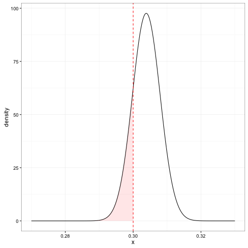
We can see that there is a nonzero probability (shaded) that his true probability of hitting is less than .3. We can calulate this with the cumulative distribution function (CDF) of the beta distribution, which in R is computed by the pbeta function:
career_eb %>% filter(name == "Hank Aaron")## Source: local data frame [1 x 8]
##
## playerID name H AB average eb_estimate alpha1 beta1
## (chr) (chr) (int) (int) (dbl) (dbl) (dbl) (dbl)
## 1 aaronha01 Hank Aaron 3771 12364 0.305 0.304 3850 8818pbeta(.3, 3850, 8818)## [1] 0.169This probability that he doesn’t belong in the Hall of Fame is called the Posterior Error Probability, or PEP. We could easily have calculated the probability Aaron does belong, which we would call the Posterior Inclusion Probability, or PIP. (Note that \(\mbox{PIP}=1-\mbox{PEP}\)) The reason we chose to measure the PEP rather than the PIP will become clear in the next section.
It’s equally straightforward to calculate the PEP for every player, just like we calculated the credible intervals for each player in the last post:
career_eb <- career_eb %>%
    mutate(PEP = pbeta(.3, alpha1, beta1))
What does the distribution of the PEP look like across players?
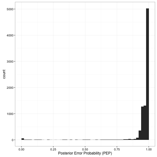
Unsurprisingly, for most players, it’s almost certain that they don’t belong in the hall of fame: we know that their batting averages are below .300. If they were included, it is almost certain that they would be an error. In the middle are the borderline players: the ones where we’re not sure. And down there close to 0 are the rare but proud players who we’re (almost) certain belong in the hall of fame.
The PEP is closely related to the estimated batting average:
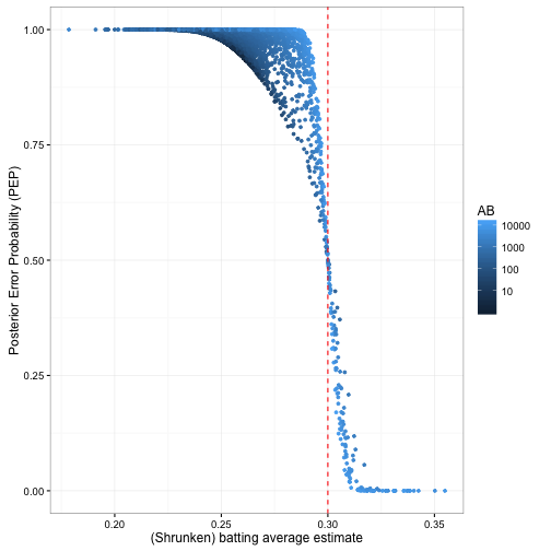
Notice that crossover point: to have a PEP less than 50%, you need to have a shrunken batting average greater than .3. That’s because the shrunken estimate is the center of our posterior beta distribution (the “over/under” point). If a player’s shrunken estimate is above .3, it’s more likely than not that their true average is as well. And the players we’re not sure about (PEP \(\approx\) .5) have batting averages very close to .300.
Notice also the relationship between the number of at-bats (the amount of evidence) and the PEP. If a player’s shrunken batting average is .28, but he hasn’t batted many times, it is still possible his true batting average is above .3- the credible interval is wide. However, if the player with .28 has a high AB (light blue), the credible interval becomes thinner, we become confident that the true probability of hitting is under .3, and the PEP goes up to 1.
False Discovery Rate
Now we want to set some threshold for inclusion in our Hall of Fame. This criterion is up to us: what kind of goal do we want to set? There are many options, but let me propose one: let’s try to include as many players as possible, while ensuring that no more than 5% of the Hall of Fame was mistakenly included. Put another way, we want to ensure that if you’re in the Hall of Fame, the probability you belong there is at least 95%.
This criterion is called false discovery rate control. It’s particularly relevant in scientific studies, where we might want to come up with a set of candidates (e.g. genes, countries, individuals) for future study. There’s nothing special about 5%: if we wanted to be more strict, we could choose the same policy, but change our desired FDR to 1% or .1%. Similarly, if we wanted a broader set of candidates to study, we could set an FDR of 10% or 20%.
Let’s start with the easy cases. Who are the players with the lowest posterior error probability?
| rank | name | H | AB | eb_estimate | PEP |
|---|---|---|---|---|---|
| 1 | Rogers Hornsby | 2930 | 8173 | 0.355 | 0 |
| 2 | Ed Delahanty | 2596 | 7505 | 0.343 | 0 |
| 3 | Shoeless Joe Jackson | 1772 | 4981 | 0.350 | 0 |
| 4 | Willie Keeler | 2932 | 8591 | 0.338 | 0 |
| 5 | Nap Lajoie | 3242 | 9589 | 0.336 | 0 |
| 6 | Tony Gwynn | 3141 | 9288 | 0.336 | 0 |
| 7 | Harry Heilmann | 2660 | 7787 | 0.339 | 0 |
| 8 | Lou Gehrig | 2721 | 8001 | 0.337 | 0 |
| 9 | Billy Hamilton | 2158 | 6268 | 0.340 | 0 |
| 10 | Eddie Collins | 3315 | 9949 | 0.331 | 0 |
These players are a no-brainer for our Hall of Fame: there’s basically no risk in including them. But suppose we instead tried to include the top 100. What do the 90th-100th players look like?
| rank | name | H | AB | eb_estimate | PEP |
|---|---|---|---|---|---|
| 90 | Stuffy McInnis | 2405 | 7822 | 0.306 | 0.134 |
| 91 | Bob Meusel | 1693 | 5475 | 0.307 | 0.138 |
| 92 | Rip Radcliff | 1267 | 4074 | 0.307 | 0.144 |
| 93 | Mike Piazza | 2127 | 6911 | 0.306 | 0.146 |
| 94 | Denny Lyons | 1333 | 4294 | 0.307 | 0.150 |
| 95 | Robinson Cano | 1649 | 5336 | 0.306 | 0.150 |
| 96 | Don Mattingly | 2153 | 7003 | 0.305 | 0.157 |
| 97 | Taffy Wright | 1115 | 3583 | 0.307 | 0.168 |
| 98 | Hank Aaron | 3771 | 12364 | 0.304 | 0.170 |
| 99 | John Stone | 1391 | 4494 | 0.306 | 0.171 |
| 100 | Ed Morgan | 879 | 2810 | 0.308 | 0.180 |
OK, so these players are borderline. We would guess that their career batting average is greater than .300, but we aren’t as certain.
So let’s say we chose to take the top 100 players for our Hall of Fame (thus, cut it off at Ed Morgan). What would we predict the false discovery rate to be? That is, what fraction of these 100 players would be falsely included?
top_players <- career_eb %>%
    arrange(PEP) %>%
    head(100)
Well, we know the PEP of each of these 100 players, which is the probability that that individual player is a false positive. And by the wonderful property of linearity of expected value, we can just add up these probabilities to get the expected value (the average) of the total number of false positives.
sum(top_players$PEP)## [1] 4.43This means that of these 100 players, we expect that about four and a half of them are false discoveries. (If it’s not clear why you can add up the probabilities like that, check out this explanation of linearity of expected value). Now, we don’t know which four or five players we are mistaken about! (If we did, we could just kick them out of the hall). But we can make predictions about the players in aggregate. Here, we can see that taking the top 100 players would get pretty close to our goal of FDR = 5%.
Note that we’re calculating the FDR as \(4.43 / 100=4.43\%\). Thus, we’re really computing the mean PEP: the average Posterior Error Probability.
mean(top_players$PEP)## [1] 0.0443We could have asked the same thing about the first 50 players, or the first 200:
sorted_PEP <- career_eb %>%
    arrange(PEP)

mean(head(sorted_PEP$PEP, 50))
## [1] 0.000992mean(head(sorted_PEP$PEP, 200))## [1] 0.238We can experiment with many thresholds to get our desired FDR, but it’s even easier just to compute them all at once, by computing the cumulative mean of all the (sorted) posterior error probabilities. We can use the cummean function from dplyr:
career_eb <- career_eb %>%
    arrange(PEP) %>%
    mutate(qvalue = cummean(PEP))
Q-values
Notice that I called the cumulative mean of the FDR a qvalue. The term q-value was first defined by John Storey as an analogue to the p-value for controlling FDRs in multiple testing. The q-value is convenient because we can say “to control the FDR at X%, collect only hypotheses where \(q < X\)”.
hall_of_fame <- career_eb %>%
    filter(qvalue < .05)
This ends up with 103 players in the Hall of Fame. If we wanted to be more careful about letting players in, we’d simply set a stricter q-value threshold:
strict_hall_of_fame <- career_eb %>%
    filter(qvalue < .01)
At which point we’d include only 68 players. It’s useful to look at how many players would be included at various thresholds:
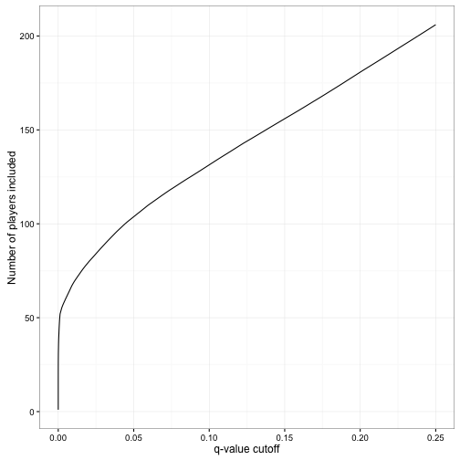
This shows that you could include 200 players in the Hall of Fame, but at that point you’d expect that about 25% of them would be incorrectly included. On the other side, you could create a hall of 50 players and be very confident that all of them have a batting probability of .300.
It’s worth emphasizing the difference between measuring an individual’s posterior error probability and the q-value, which is the false discovery rate of a group including that player. Hank Aaron has a PEP of 17%, but he can be included in the Hall of Fame while keeping the FDR below 5%. If this is surprising, imagine that you were instead trying to keep the average height above 6’0”. You would start by including all players taller than 6’0”, but could also include some players who were 5’10” or 5’11” while preserving your average. Similarly, we simply need to keep the average PEP of the players below 5%. (For this reason, the PEP is sometimes called the local false discovery rate, which emphasizes both the connection and the distinction).
Frequentists and Bayesians; meeting in the middle
In my previous three posts, I’ve been taking a Bayesian approach to our estimation and interpretation of batting averages. We haven’t really used any frequentist statistics: in particular, we haven’t seen a single p-value or null hypothesis. Now we’ve used out posterior distributions to compute q-values, and used it to control false discovery rate.
But note that the q-value was originally defined in terms of null hypothesis significance testing, particularly as a transformation of p-values under multiple testing. By calculating, and then averaging, the posterior error probability, we’ve found another way to control FDR. This connection is explored in two great papers from my former advisor, found here and here.
There are some notable differences between our approach here and typical FDR control. In particular, we aren’t defining a null hypothesis (we aren’t assuming any players have a batting average equal to .300), but are instead trying to avoid what Andrew Gelman calls “Type S errors”. Still, this is another great example of the sometimes underappreciated technique of examining the frequentist properties of Bayesian approaches- and, conversely, understanding the Bayesian interpretations of frequentist goals.
What’s Next: A/B testing of batters
We’ve been comparing each player to a fixed threshold, .300. What if we want to compare two players to each other? For instance, catcher Mike Piazza has a higher career batting average (2127 / 6911 = 0.308) than Hank Aaron (3771 / 12364 = 0.305). Can we say with confidence that his true batting average is higher?
This is the common problem of comparing two proportions, which often occurs in A/B testing (e.g. comparing two versions of an login form to see which gets a higher signup rate). We’ll apply some of what we learned here about the Bayesian approach to hypothesis testing, and see how sharing information across batters with empirical Bayes can once again give us an advantage.