Previously in this series:
- The “lost boarding pass” puzzle
- The “deadly board game” puzzle
- The “knight on an infinite chessboard” puzzle
- The “largest stock profit or loss” puzzle
The birthday problem is a classic probability puzzle, stated something like this.
A room has n people, and each has an equal chance of being born on any of the 365 days of the year. (For simplicity, we’ll ignore leap years). What is the probability that two people in the room have the same birthday?
If you’re not familiar with the puzzle, you might expect that in a moderately sized room (like 20-30 people) that the chance will be pretty small that two people have the same birthday. But in fact, if the room has more than 23 people, the chance is greater than 50%! This makes the puzzle a classic for intro statistics classes.
I’ve been interested for a while in the tidyverse approach to simulation. In this post, I’ll use the birthday problem as an example of this kind of tidy simulation, most notably the use of the underrated crossing() function.
Simulating the birthday paradox
First, I’ll show the combined approach, before breaking it down.
library(tidyverse)
theme_set(theme_light())

summarized <- crossing(people = seq(2, 50, 2),
                       trial = 1:10000) %>%
  mutate(birthday = map(people, ~ sample(365, ., replace = TRUE)),
         multiple = map_lgl(birthday, ~ any(duplicated(.)))) %>%
  group_by(people) %>%
  summarize(chance = mean(multiple))

# Visualizing the probability
ggplot(summarized, aes(people, chance)) +
  geom_line() +
  scale_y_continuous(labels = scales::percent_format()) +
  labs(y = "Probability two have the same birthday")
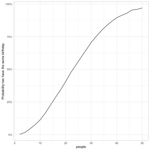
This visualization shows that the probability two people have the same birthday is low if there are 10 people in the room, moderate if there are 10-40 people in the room, and very high if there are more than 40. It crosses over to become more likely than not when there are ~23 people in the room.
I’ll break down the simulation a bit below.
Simulating one case
When you’re approaching a simulation problem, it can be worth simulating a single case first.
Suppose we have 20 people in a room. Ignoring leap years (and treating each calendar day as a number from 1 to 365), we can simulate their birthdays with sample(365, 20, replace = TRUE).
# 10 random numbers from 1 to 365
sample(365, 10, replace = TRUE)
## [1] 53 216 220 309 13 37 35 299 263 333We then use two handy base R functions, duplicated and any, to discover if there are any duplicated days.
# When the values 2 and 1 appear for the second time, they're TRUE
duplicated(c(1, 2, 3, 4, 2, 5, 1))
## [1] FALSE FALSE FALSE FALSE TRUE FALSE TRUE# This asks "are any values here duplicated?"
any(duplicated(c(1, 2, 3, 4, 2, 5, 1)))## [1] TRUEThis gives us a one-liner for simulating a single case of the birthday problem, with (say) 20 people:
any(duplicated(sample(365, 20, replace = TRUE)))## [1] TRUEIf you run this line a few times, you’ll see it’s sometimes true and sometime false, which already gives us the sense that pairs of people sharing a birthday in a moderately-sized room aren’t as rare as you might expect.
The tidy approach to many simulations across multiple parameters
I find the crossing() function in tidyr incredibly valuable for simulation. crossing() creates a tibble of all combinations of its arguments.
crossing(first = c("a", "b", "c"),
         second = c(1, 2, 3))
## # A tibble: 9 x 2
## first second
## <chr> <dbl>
## 1 a 1
## 2 a 2
## 3 a 3
## 4 b 1
## 5 b 2
## 6 b 3
## 7 c 1
## 8 c 2
## 9 c 3Our simulation starts by generating 10000 * 25 combinations of people and trial, with values of people ranging from 2 to 50. trial exists only so that we have many observations of each, in order to minimize statistical noise.
# Generate combinations of 10,000 replications and number of people (2-50)
crossed <- summarized <- crossing(trial = seq_len(10000),
                                  people = seq(2, 50, 2))

crossed
## # A tibble: 250,000 x 2
## trial people
## <int> <dbl>
## 1 1 2
## 2 1 4
## 3 1 6
## 4 1 8
## 5 1 10
## 6 1 12
## 7 1 14
## 8 1 16
## 9 1 18
## 10 1 20
## # … with 249,990 more rowsWe then use functions from purrr, useful for operating across a list, to generate a list column of integer vectors. With a second step, we determine which of them have multiples of any birthday.
# Generate a list column of samples
sim <- crossed %>%
  mutate(birthday = map(people, ~ sample(365, ., replace = TRUE)),
         multiple = map_lgl(birthday, ~ any(duplicated(.))))

sim
## # A tibble: 250,000 x 4
## trial people birthday multiple
## <int> <dbl> <list> <lgl>
## 1 1 2 <int [2]> FALSE
## 2 1 4 <int [4]> FALSE
## 3 1 6 <int [6]> TRUE
## 4 1 8 <int [8]> FALSE
## 5 1 10 <int [10]> FALSE
## 6 1 12 <int [12]> FALSE
## 7 1 14 <int [14]> FALSE
## 8 1 16 <int [16]> FALSE
## 9 1 18 <int [18]> FALSE
## 10 1 20 <int [20]> FALSE
## # … with 249,990 more rowsFinally, we use one of my favorite tricks in R: using mean() to find the fraction of a logical vector that’s TRUE.
# Find the percentage of cases where multiple is TRUE
summarized <- sim %>%
  group_by(people) %>%
  summarize(chance = mean(multiple))

summarized
## # A tibble: 25 x 2
## people chance
## <dbl> <dbl>
## 1 2 0.0019
## 2 4 0.0157
## 3 6 0.0434
## 4 8 0.0706
## 5 10 0.113
## 6 12 0.162
## 7 14 0.223
## 8 16 0.279
## 9 18 0.344
## 10 20 0.414
## # … with 15 more rowsTogether these three steps (crossed+sim+summarized) make up the solution in the first code chunk above. Notice this simulation combines the base R approach (sample, duplicated, and any) with tidyverse functions from dplyr (like mutate, group_by, and summarize), tidyr (crossing) and purrr (map and map_lgl). I’ve found this crossing/map/summarize approach useful in many simulations.
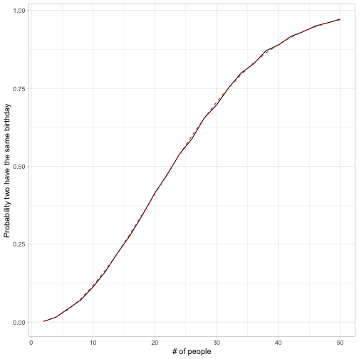
How can we check our math? R has a built-in pbirthday function that gives an exact solution: for instance, pbirthday(20) gives the probability two people in a room of 20 will have the same birthday. We can compare our su
# pbirthday is not vectorized, so we have to use map_dbl
summarized %>%
  mutate(exact = map_dbl(people, pbirthday)) %>%
  ggplot(aes(people, chance)) +
  geom_line() +
  geom_line(aes(y = exact), lty = 2, color = "red") +
  labs(x = "# of people",
       y = "Probability two have the same birthday")
Looks like we got very close!
Generalizing the birthday problem
We’ve seen how likely it is that there’s a pair of people with the same birthday. What about a group of 3, 4, or 5 who all have the same birthday? How likely is that?
First, instead of working with ~ any(duplicated(.)) as our vectorized operation, we could find how many people are in the most common group of birthdays, with another combination of base R functions: max and table.
# table() returns a vector of frequencies
table(c("a", "b", "b", "c", "c", "d", "d", "d"))
##
## a b c d
## 1 2 2 3# So max(table()) tells us that in this group, one letter occurs 3 times
max(table(c("a", "b", "b", "c", "c", "d", "d", "d")))## [1] 3# Use this max(table()) approach in the map_int
sim_most_common <- crossing(people = seq(5, 100, 5),
trial = 1:5000) %>%
mutate(birthday = map(people, ~ sample(365, ., replace = TRUE))) %>%
mutate(most_common = map_int(birthday, ~ max(table(.))))
sim_most_common## # A tibble: 100,000 x 4
## people trial birthday most_common
## <dbl> <int> <list> <int>
## 1 5 1 <int [5]> 1
## 2 5 2 <int [5]> 1
## 3 5 3 <int [5]> 1
## 4 5 4 <int [5]> 1
## 5 5 5 <int [5]> 1
## 6 5 6 <int [5]> 1
## 7 5 7 <int [5]> 1
## 8 5 8 <int [5]> 1
## 9 5 9 <int [5]> 2
## 10 5 10 <int [5]> 1
## # … with 99,990 more rowsNow that we know within each trial what the largest group with the same birthday is. We now need to know the fraction within each number where the most_common is at least 2, 3, 4, or 5. We use another application of the ever-useful crossing function, to apply multiple thresholds to each number of people.
summarized_most_common <- sim_most_common %>%
  crossing(threshold = 2:5) %>%
  group_by(people, threshold) %>%
  summarize(chance = mean(most_common >= threshold))

summarized_most_common
## # A tibble: 80 x 3
## # Groups: people [20]
## people threshold chance
## <dbl> <int> <dbl>
## 1 5 2 0.0302
## 2 5 3 0
## 3 5 4 0
## 4 5 5 0
## 5 10 2 0.115
## 6 10 3 0.001
## 7 10 4 0
## 8 10 5 0
## 9 15 2 0.250
## 10 15 3 0.0036
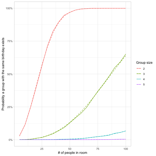
## # … with 70 more rowsWe can visualize these and compare them to the exact values from pbirthday() (pbirthday() takes a coincident argument to extend the problem to more than two participants).
summarized_most_common %>%
  mutate(exact = map2_dbl(people, threshold,
                          ~ pbirthday(.x, coincident = .y))) %>%
  ggplot(aes(people, chance, color = factor(threshold))) +
  geom_line() +
  geom_line(aes(y = exact), lty = 2) +
  scale_y_continuous(labels = scales::percent_format()) +
  labs(x = "# of people in room",
       y = "Probability a group with the same birthday exists",
       color = "Group size")
From this we learn that in a room of 100 people, it is almost certain that a pair exists with the same birthday, more likely than not that that a group of 3 does, unlikely that a group of 4 does, and almost impossible that a group of 5 does.
What I like about the tidy approach to simulation is that we can keep adding parameters that we’d like to vary through an extra crossing() and an extra term in the group_by. For instance, if we’d wanted to see how the probability varied as the number of days in a year changed (not relevant for birthdays, but might be relevant in other applications like the cryptographic birthday attack), we could have added that to the crossing() and worked with the first argument to sample.
