
Previously in this series:
- The “lost boarding pass” puzzle
- The “deadly board game” puzzle
- The “knight on an infinite chessboard” puzzle
- The “largest stock profit or loss” puzzle
- The “birthday paradox” puzzle
I have an interest in probability puzzles and riddles, and especially in simulating them in R. I recently learned about Feller’s coin-tossing puzzle, from the book Mathematical Constants by Steven Finch. (I recommend the book if you like the topic too!)
Mathematician William Feller posed the following problem:
If you flip a coin \(n\) times, what is the probability there are no streaks of \(k\) heads in a row?
Note that while the number of heads in a sequence is governed by the binomial distribution, the presence of consecutive heads is a bit more complicated, because the presence of a streak at various points in the sequence isn’t independent. This reminds me a bit of one of my earlier tidyverse simulations:
A #tidyverse simulation to demonstrate that if you wait for two heads in a row, it takes 6 flips on average, while you wait for a heads then a tails, it takes 4 flips on average
— David Robinson (@drob) June 17, 2018
h/t @CutTheKnotMath #rstats pic.twitter.com/V0zgOmCy7t
To continue my series of simulating probability puzzles in the tidyverse, I’d like to show how we’d approach simulating Feller’s coin-tossing problem, and comparing it to the exact values. (In the process, we also see how we’d calculate a Fibonacci sequence in one line!)
Simulating a single sequence
Let’s start with values \(n=20;k=3\): what’s the probability that a sequence of 20 flips contains no streaks of length 3? You can flip a sequence of coins with rbinom().
# We'll say 1 is heads, 0 is tails
flips <- rbinom(20, 1, .5)
flips
## [1] 1 0 0 0 1 0 1 1 1 0 1 1 1 1 1 0 0 1 1 1In this case, there were indeed a few streaks of 3 heads in a row. How could determine that in R?
Well, we could use dplyr’s window function lead() (which moves each flip forward one in the sequence), to ask if there are any flips sets in which a coin, the next coin, and the one after that are all 1 (heads).
library(dplyr)

flips & lead(flips) & lead(flips, 2)
## [1] FALSE FALSE FALSE FALSE FALSE FALSE TRUE FALSE FALSE FALSE TRUE
## [12] TRUE TRUE FALSE FALSE FALSE FALSE TRUE NA NAIndeed, there are (though notice the last two are NA, since there is no lead() coin).
Remember that Feller was looking for the probability there are no streaks in the sequence. We use !any() to check this:
!any(flips & lead(flips) & lead(flips, 2), na.rm = TRUE)## [1] FALSEThis gives us an approach that, similar to our previous tidyverse approaches to simulation, we can repeat and summarize across parameter values using tidyr’s crossing() and purrr’s map_lgl().
library(tidyverse)

# Set up a function for there being no streak of 3
no_three_heads <- function(x) {
  !any(x & lead(x) & lead(x, 2), na.rm = TRUE)
}

# Note that if there are 1 or 2 flips, the probability is 100%
sim <- crossing(trial = seq_len(10000),
                sequence_length = seq(3, 51, 2)) %>%
  mutate(flips = map(sequence_length, rbinom, 1, .5)) %>%
  mutate(no_three = map_lgl(flips, no_three_heads)) %>%
  group_by(sequence_length) %>%
  summarize(chance_no_three = mean(no_three))

sim
## # A tibble: 25 x 2
## sequence_length chance_no_three
## <dbl> <dbl>
## 1 3 0.874
## 2 5 0.744
## 3 7 0.635
## 4 9 0.528
## 5 11 0.452
## 6 13 0.387
## 7 15 0.323
## 8 17 0.280
## 9 19 0.230
## 10 21 0.193
## # … with 15 more rowsThis takes about 5 seconds on my machine. We can then visualize the probability that there are no streaks as a function of the number of flips in the sequence.
ggplot(sim, aes(sequence_length, chance_no_three)) +
  geom_line() +
  scale_y_continuous(labels = scales::percent_format()) +
  labs(x = "# of flips",
       y = "Probability there are no sequences of 3 heads")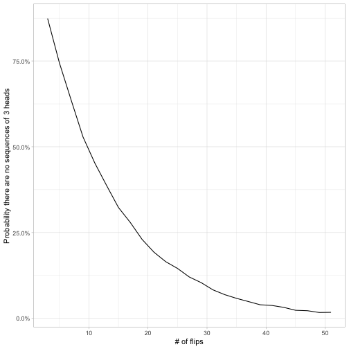
It looks like for \(k=3\), the probability there are no sequences of three is 7/8 for a sequence of 3 flips, crosses 50% roughly when there are 10 flips, and then is rather close to zero by the time there are 50 flips.
Extending for multiple values of k
Once we’re not fixed to \(k=3\), we can’t use x & lead(x) & lead(x, 2) to check for the presence of a streak anymore.1 As a replacement, I’d like to introduce a useful base R function called rle, for “run-length encoding”.
rle(flips)## Run Length Encoding
## lengths: int [1:9] 1 3 1 1 3 1 5 2 3
## values : int [1:9] 1 0 1 0 1 0 1 0 1A run-length encoding divides a vector down into streaks of consecutive values. It turns the vector into two components: the lengths of each streak, and the value in each. We can use these in combination- !any(r$values & r$lengths >= len)- to check if there are any streaks of heads greater than a certain length. (This is a good example of how knowing slightly obscure base R functions, like rle, gives you a toolbox for elegant and efficient solutions).
By adding a value k to our crossing(), we can then visualize the probability for each value of k.
no_streak <- function(x, len) {
  r <- rle(x)
  !any(r$values & r$lengths >= len)
}

# Note that when k is 1, the probability is 2^(-n), not too exciting
feller_seq <- crossing(trial = seq_len(10000),
                       n = seq(2, 40, 2),
                       k = 2:4) %>%
  mutate(flips = map(n, rbinom, 1, .5)) %>%
  mutate(no_seq = map2_lgl(flips, k, no_streak)) %>%
  group_by(n, k) %>%
  summarize(p = mean(no_seq))

feller_seq
## # A tibble: 60 x 3
## # Groups: n [20]
## n k p
## <dbl> <int> <dbl>
## 1 2 2 0.751
## 2 2 3 1
## 3 2 4 1
## 4 4 2 0.497
## 5 4 3 0.811
## 6 4 4 0.934
## 7 6 2 0.337
## 8 6 3 0.692
## 9 6 4 0.869
## 10 8 2 0.214
## # … with 50 more rowsfeller_seq %>%
ggplot(aes(n, p, color = factor(k))) +
geom_line() +
scale_y_continuous(labels = scales::percent) +
labs(y = "Probability there is no streak",
color = "Length of streak")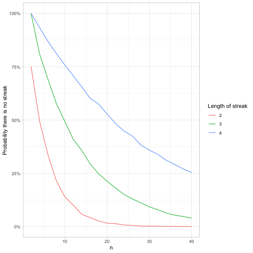
The longer the streak, the less likely the sequence won’t contain it, which makes sense. By the time the sequence is length 40, it’s almost certain to contain a stretch of 2 heads, very likely to contain a stretch of 3 heads, and has a 75% chance to contain a stretch of 4 heads.
Feller’s coin-tossing constants
Something I like about simulations is that they can double-check mathematical results.
When Feller looked at this problem, he proved a result about \(p(n,k)\), namely:
\[\lim_{n\rightarrow \infty}\alpha_k p(n, k)=\beta_k\]Where \(\alpha_k\) and \(\beta_k\) are Feller’s constants. (You can find a few such values, and some more details, on Wikipedia). We could compare those exact values to the simulation, by creating a table of the constants and joining them.
feller_constants <- tibble(k = c(2, 3, 4),
                           alpha = c(1.236, 1.087, 1.0376),
                           beta = c(1.447, 1.237, 1.137))

feller_seq %>%
  inner_join(feller_constants, by = "k") %>%
  ggplot(aes(n)) +
  geom_line(aes(y = p, color = factor(k))) +
  geom_line(aes(y = beta / alpha ^ (n + 1), group = k), lty = 2) +
  scale_y_continuous(labels = scales::percent) +
  labs(x = "Length of sequence",
       y = "Probability there is no streak of heads",
       color = "Length of streak")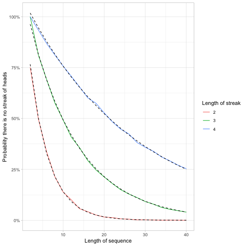
Calculating the probability of Fibonacci numbers
But an approach I like even more than Feller’s constants is to calculate the exact probability based on higher-order Fibonacci sequences.
\[p(n,k)=\frac{F^{(k)}_{n + 2}}{2^n}\]where \(F^{(k)}_{n + 2}\) is the \(n+2\) term of the \(k\)th order Fibonacci sequence. The first few paragraphs of this paper points out why. (In short for \(k=2\): the number of sequences of length \(n\) that have no streaks of 2 is all the sequences of length \(n-1\) that are followed by a \(T\), plus all the sequences of length \(n-2\) that are followed by a \(TH\). This is divided by the \(2^n\) possible sequences.)
Let’s talk about Fibonacci sequences! Each step in a Fibonacci sequence is the sum of the previous 2, after starting with (1, 1). To get that in R, you’d keep applying the step c(., sum(tail(., 2))) again and again (tail() gets the last items of a vector).
This can be done in one line (trick of the day!) with the reduce function from purrr, which calls a function for each element in a vector while passing along the result. When passed a dummy vector, like 1:50, and an initial value, like c(1, 1) (the first two), it’s a quick way to say “call this function 50 times”.
# Gets the first 52 fibonacci numbers, starting with 1, 1
reduce(seq_len(50), ~ c(., sum(tail(., 2))), .init = c(1, 1))
## [1] 1 1 2 3 5
## [6] 8 13 21 34 55
## [11] 89 144 233 377 610
## [16] 987 1597 2584 4181 6765
## [21] 10946 17711 28657 46368 75025
## [26] 121393 196418 317811 514229 832040
## [31] 1346269 2178309 3524578 5702887 9227465
## [36] 14930352 24157817 39088169 63245986 102334155
## [41] 165580141 267914296 433494437 701408733 1134903170
## [46] 1836311903 2971215073 4807526976 7778742049 12586269025
## [51] 20365011074 32951280099In higher order Fibonacci sequences, the terms are the sum of 3 (“tribonacci”), 4 (“tetranacci”), or more previous terms, meaning they grow even faster. We could create a function that calculates those series.
fibonacci <- function(order) {
  reduce(seq_len(50), ~ c(., sum(tail(., order))), .init = c(1, 1))
}

# Fibonacci
head(fibonacci(2))
## [1] 1 1 2 3 5 8# Tribonacci
head(fibonacci(3))## [1] 1 1 2 4 7 13So returning to our simulation, we can confirm our math.
feller_seq %>%
  group_by(k) %>%
  mutate(exact = fibonacci(k[1])[n + 2] / 2 ^ n) %>%
  ggplot(aes(n)) +
  geom_line(aes(y = p, color = factor(k))) +
  geom_line(aes(y = exact, group = k), lty = 2) +
  scale_y_continuous(labels = scales::percent) +
  labs(y = "Probability there is no streak",
       color = "Length of streak")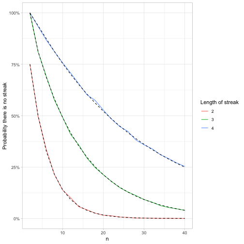
Notice what a wide range of tools can be used in simulations. Besides our usual collection of tidyverse tricks like crossing(), we used rle() (a handy trick any time you need to examine consecutive streaks), and reduce() (useful for setting up recursive relationships like in the Fibonacci sequence).
I’m really enjoying these probability puzzle simulations. If you have a favorite probability puzzle you’d like me to simulate, please put in the comments!
-
With
reduce, there actually is a way we could take thelead()approach with an arbitrary streak length (left as an exercise to the reader!). But I found it’s about 10X slower than therle()approach above, so I’m focusing on this one. ↩