Previously in this series:
- Understanding the beta distribution
- Understanding empirical Bayes estimation
- Understanding credible intervals
- Understanding the Bayesian approach to false discovery rates
- Understanding Bayesian A/B testing
- Understanding beta binomial regression
Suppose you were a scout hiring a new baseball player, and were choosing between two that have had 100 at-bats each:
- A left-handed batter who has hit 30 hits / 100 at-bats
- A right-handed batter who has hit 30 hits / 100 at-bats
Who would you guess was the better batter?
This seems like a silly question: they both have the same exact batting record. But what if I told you that historically, left-handed batters are slightly better hitters than right-handed? How could you incorporate that evidence?
In the last post, we used the method of beta binomial regression to incorporate information (specifically the number of at-bats a player had) into a per-player prior distribution. We did this to correct a bias of the algorithm, but we could do a lot with this method: in particular, we can include other factors that might change our prior expectations of a player.
These are particular applications of Bayesian hierarchical modeling, where the priors for each player are not fixed, but rather depend on other latent variables. In our empirical Bayesian approach to hierarchical modeling, we’ll estimate this prior using beta binomial regression, and then apply it to each batter. This strategy is useful in many applications beyond baseball- for example, if I were analyzing ad clickthrough rates on a website, I may notice that different countries have different clickthrough rates, and therefore fit different priors for each. This could influence our Bayesian A/B tests, credible intervals, and more.
Setup
As usual, I’ll start with some code you can use to catch up if you want to follow along in R. If you want to understand what it does in more depth, check out the previous posts in this series. (As always, all the code in this post can be found here).
library(gamlss)
library(dplyr)
library(tidyr)
library(Lahman)
library(ggplot2)
theme_set(theme_bw())

# Grab career batting average of non-pitchers
# (allow players that have pitched <= 3 games, like Ty Cobb)
pitchers <- Pitching %>%
  group_by(playerID) %>%
  summarize(gamesPitched = sum(G)) %>%
  filter(gamesPitched > 3)

# in this setup, we're keeping some extra information for later in the post:
# a "bats" column and a "year" column
career <- Batting %>%
  filter(AB > 0) %>%
  anti_join(pitchers, by = "playerID") %>%
  group_by(playerID) %>%
  summarize(H = sum(H), AB = sum(AB), year = mean(yearID)) %>%
  mutate(average = H / AB)

# Add player names
career <- Master %>%
  tbl_df() %>%
  dplyr::select(playerID, nameFirst, nameLast, bats) %>%
  unite(name, nameFirst, nameLast, sep = " ") %>%
  inner_join(career, by = "playerID")
Based on our last post, we perform beta binomial regression using the gamlss package. This fits a model that allows the mean batting average \(\mu\) to depend on the number of at-bats a player has had.
library(gamlss)

fit <- gamlss(cbind(H, AB - H) ~ log(AB),
              data = dplyr::select(career, -bats),
              family = BB(mu.link = "identity"))
The prior \(\alpha_0\) and \(\beta_0\) can then be computed for each player based on \(\mu\) and a dispersion parameter \(\sigma\):
career_eb <- career %>%
  mutate(mu = fitted(fit, "mu"),
         sigma = fitted(fit, "sigma"),
         alpha0 = mu / sigma,
         beta0 = (1 - mu) / sigma,
         alpha1 = alpha0 + H,
         beta1 = beta0 + AB - H,
         estimate = alpha1 / (alpha1 + beta1))
Now we’ve corrected for one confounding factor, \(\mbox{AB}\). One important aspect of this prediction is that it won’t be useful when we’ve just hired a “rookie” player, and we’re wondering what his batting average will be. This observed variable \(\mbox{AB}\) is based on a player’s entire career, such that a low number is evidence that a player didn’t have much of a chance to bat. (If we wanted to make a prediction, we’d have to consider the distribution of possible \(\mbox{AB}\)’s the player could end up with and integrate over that, which is beyond the scope of this post).
But there’s some information we can use even at the start of a player’s career. Part of the philosophy of the Bayesian approach is to bring our prior expectations in mathematically. Let’s try doing that with some factors that influence batting success.
Right- and left- handed batters
It’s well known in sabermetrics that left-handed batters tend to bat slightly better. (In fact, the general belief is that left-handed batters have an advantage against right-handed pitchers, but since most pitchers historically have been right-handed this evens out to an advantage). The Lahman dataset provides that information in the bats column: in the above code, I retained it as part of the career dataset.
career %>%
  count(bats)
## # A tibble: 4 × 2
## bats n
## <fctr> <int>
## 1 B 815
## 2 L 2864
## 3 R 5869
## 4 NA 840These letters represent “Both” (switch hitters), “Left”, and “Right”, respectively. One interesting feature is that while the ratio of righties to lefties is about 9-to-1 in the general population, in professional baseball it is only 2-to-1. Managers like to hire left-handed batters- in itself, this is some evidence of a left-handed advantage! We also see that there are a number of batters (mostly from earlier in the game’s history) that we don’t have handedness information for. We’ll filter them out of this analysis.
Incorporating this as a predictor is as simple as adding bats to the formula in the gamlss call (our beta-binomial regression):
# relevel to set right-handed batters as the baseline
career2 <- career %>%
  filter(!is.na(bats)) %>%
  mutate(bats = relevel(bats, "R"))

fit2 <- gamlss(cbind(H, AB - H) ~ log(AB) + bats,
               data = career2,
               family = BB(mu.link = "identity"))
We can then look at the coefficients:
library(broom)
tidy(fit2)
## parameter term estimate std.error statistic p.value
## 1 mu (Intercept) 0.14077 0.001626 86.6 0.00e+00
## 2 mu log(AB) 0.01516 0.000219 69.1 0.00e+00
## 3 mu batsB -0.00108 0.000990 -1.1 2.73e-01
## 4 mu batsL 0.01011 0.000634 15.9 1.75e-56
## 5 sigma (Intercept) -6.37789 0.023299 -273.7 0.00e+00According to our beta-binomial regression, there is indeed a statistically significant advantage to being left-handed, with lefties hitting about 1% more often. This may seem like a small effect, but over the course of multiple games it could certainly make a difference. In contrast, there’s apparently no detectable advantage to being able to bat with both hands. (This surprised me- does anyone know a reason this might be?)
For our empirical Bayes estimation, this means every combination of handedness and AB now has its own prior:
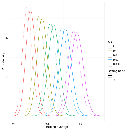
We can use these priors to improve our estimates of each player, by effectively giving a natural advantage to each left-handed batter. Note that this prior can still easily be overcome by enough evidence. For example, consider our hypothetical pair of battters from the introduction, where each has a 30% success rate, but where one is left-handed and one right-handed. If the batters had few at-bats, we’d guess that the left-handed batter was better, but the posterior for the two will converge as AB increases:
crossing(bats = c("L", "R"),
         AB = c(10, 100, 1000, 10000)) %>%
  augment(fit2, newdata = .) %>%
  mutate(H = .3 * AB,
         alpha0 = .fitted / sigma,
         beta0 = (1 - .fitted) / sigma,
         alpha1 = alpha0 + H,
         beta1 = beta0 + AB - H,
         estimate = alpha1 / (alpha1 + beta1),
         conf.low = qbeta(.025, alpha1, beta1),
         conf.high = qbeta(.975, alpha1, beta1),
         record = paste(H, AB, sep = " / ")) %>%
  ggplot(aes(estimate, record, color = bats)) +
  geom_point() +
  geom_errorbarh(aes(xmin = conf.low, xmax = conf.high)) +
  labs(x = "Estimate w/ 95% credible interval",
       y = "Batting record",
       color = "Batting hand")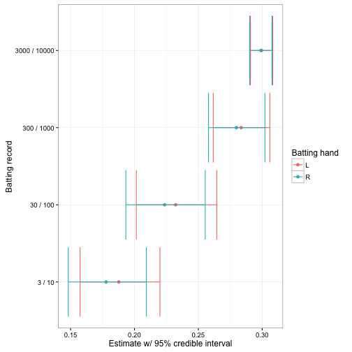
Over time
One of the most dramatic pieces of information we’ve “swept under the rug” in our analysis is the time period when each player was active. It’s absurd to expect that players in the 1880s would have the same ranges of batting averages as players today, and we should take that into account in our estimates. I thus included year = mean(yearID) in the summary of each player when I constructed this data, to summarize the time period of each player using the midpoint of their career.
Could we simply fit a linear model with respect to year (~ log10(AB) + bats + year)? Well, before we fit a model we should always look at a graph. A boxplot comparing decades is a good start (here I’m looking only at players with >= 500 AB in their career):
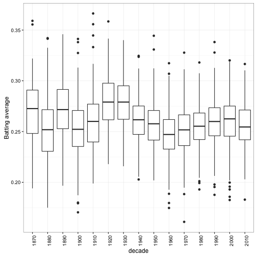
Well, there’s certainly a trend over time, but there’s nothing linear about it: batting averages have both risen and fallen across time. If you’re interested in baseball history and not just Bayesian statistics, you may notice that this graph marks the “power struggle” between offense and defense:
- The rise in the 1920s and 1930s marks the end of the dead-ball era, where hitting, especially home runs, became a more important part of the game
- The batting average “cools off” as pitchers adjust their technique, especially when the range of the strike zone was increased in 1961
- Batting average rose again in the 1970s thanks to the designated hitter rule, where pitchers (in one of the two main leagues) were no longer required to bat
- It looks like batting averages may again be drifting downward
In any case, we certainly can’t fit a simple linear trend here. We could instead fit a natural cubic spline using the ns function:1
library(splines)

fit3 <- gamlss(cbind(H, AB - H) ~ 0 + ns(year, df = 5) + bats + log(AB),
               data = career2,
               family = BB(mu.link = "identity"))
(If you’re not familiar with splines, don’t worry about them- what’s important is that even in a linear model, we can include nonlinear trends)
We now have a prior for each year, handedness, and number of at-bats. For example, here’s the distributions for a hypothetical player with AB = 1000:
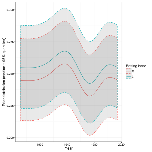
Note that those intervals don’t represent uncertainty about our trend: they represent the 95% range in prior batting averages. Each combination of year and left/right handedness is a beta distribution, of which we’re seeing just one cross-section.
One of the implicit assumptions of the above model is that the effect of left-handedness hasn’t changed over time. But this may not be true! We can change the formula to allow an interaction term ns(year, 5) * bats, which lets the effect of handedness change over time:
fit4 <- gamlss(cbind(H, AB - H) ~ 0 + ns(year, 5) * bats + log(AB),
               data = career2,
               family = BB(mu.link = "identity"))
The priors now look like:
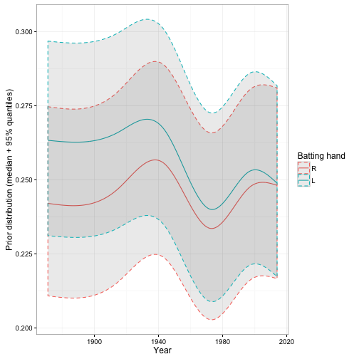
Interesting- we can now see that the gap between left-handed and right-handed batters has been closing since the start of the game, such that today the gap has basically completely disappeared. This suggests that managers and coaches may have learned how to deal with left-handed batters. Inspired by this, I might wonder if the percentage of games started by left-handed pitchers has been going up over time, and I notice that it has:
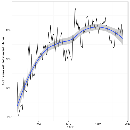
This is one thing I like about fitting hierarchical models like these- they don’t just improve your estimation, they can also give you insights into your data.
Let’s go back to those two batters with a record of 30 hits out of 100 at-bats. We’ve now seen that this would be a different question in different years. Let’s consider what it would look like in three different years, each 50 years apart:
players <- crossing(year = c(1915, 1965, 2015),
                    bats = c("L", "R"),
                    H = 30,
                    AB = 100)

players_posterior <- players %>%
  mutate(mu = predict(fit4, what = "mu", newdata = players),
         sigma = predict(fit4, what = "sigma", newdata = players, type = "response"),
         alpha0 = mu / sigma,
         beta0 = (1 - mu) / sigma,
         alpha1 = alpha0 + H,
         beta1 = beta0 + AB - H)

players_posterior
## # A tibble: 6 × 10
## year bats H AB mu sigma alpha0 beta0 alpha1 beta1
## <dbl> <chr> <dbl> <dbl> <dbl> <dbl> <dbl> <dbl> <dbl> <dbl>
## 1 1915 L 30 100 0.230 0.00141 163 545 193 615
## 2 1915 R 30 100 0.211 0.00141 150 559 180 629
## 3 1965 L 30 100 0.208 0.00141 148 561 178 631
## 4 1965 R 30 100 0.201 0.00141 142 566 172 636
## 5 2015 L 30 100 0.212 0.00141 150 558 180 628
## 6 2015 R 30 100 0.212 0.00141 150 558 180 628How do these posterior distributions (the alpha1 and beta1 we chose) differ?
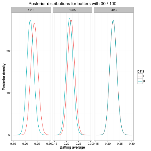
If this comparison had happened in 1915, you may have wanted to pick the left-handed batter. We wouldn’t have been sure he was better (we’d need to apply one of these methods for that), but it was more likely than not. But today, there’d be basically no reason to: left- versus right- handedness has almost no extra information.
Note: Uncertainty in hyperparameters
We’ve followed the philosophy of empirical Bayes so far: we fit hyperparameters (\(\alpha_0\), \(\beta_0\), or our coefficients for time and handedness) for our model using maximum likelihood (e.g. beta-binomial regression), and then use that as the prior for each of our observations.
Empirical Bayes in a nutshell: Estimate priors like a frequentist then carry out a Bayesian analysis.
— Data Science Fact (@DataSciFact) June 10, 2016
There’s a problem I’ve been ignoring so far with the empirical Bayesian approach, which is that there’s uncertainty in these hyperparameters as well. When we come up with an alpha and beta, or come up with particular coefficients over time, we are treating those as fixed knowledge, as if these are the priors we “entered” the experiment with. But in fact each of these parameters were chosen from this same data, and in fact each comes with a confidence interval that we’re entirely ignoring. This is sometimes called the “double-dipping” problem among critics of empirical Bayes.
This wasn’t a big deal when we were estimating just \(\alpha_0\) and \(\beta_0\) for the overall dataset: we had so much data, and were estimating so few parameters, that we could feel good about the approach. But now that we’re fitting this many parameters, we’re pushing it. Actually quantifying this, and choosing methods robust to the charge of “double-dipping”, involves Bayesian methods outside the scope of this series. But I wanted to note that this post reaches the edge of what empirical Bayes can be used for.
What’s Next: Mixture models
We’ve been treating our overall distribution of batting averages as a beta distribution. But what if that weren’t a good fit? For example, what if we had a multimodal distribution?
We’ve been filtering out pitchers during this analysis. But when we leave them in, the data looks a lot less like a beta. The dashed density curve represents the beta distribution we would naively fit to this data.
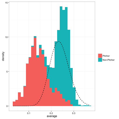
We can see that batting averages with pitchers incldued isn’t made up of a single beta distribution- it’s more like two separate ones mixed together. Imagine that you didn’t know which players were pitchers,2 and you wanted to separate the data into two groups according to your best prediction. This is very common in practical machine learning applications, such as clustering and segmentation.
In my next post I’m going to introduce mixture models, treating the distribution of batting averages as a mixture of two beta-binomial distributions and estimating which player belongs to which group. This will also introduce the concept of an expectation-maximization algorithm, which is important in both Bayesian and frequentist statistics. We’ll see that mixture models are still a good fit for the empirical Bayes framework, and show how to calculate a posterior probability for the cluster each player belongs to.
Footnotes
-
Why 5 degrees of freedom? Not very scientific- I just tried a few and picked one that roughly captured the shapes we saw in the boxplots. If you have too few degrees of freedom you can’t capture the complex trend we’re seeing here, but if you have too many you’ll overfit to noise in your data. ↩
-
Admittedly it’s not very realistic to assume we don’t know which players are pitchers. But this gives us a great example of fitting a mixture model, which will be an important element of this series. ↩
