Previously in this series:
I’ve recently been enjoying The Riddler: Fantastic Puzzles from FiveThirtyEight, a wonderful book from 538’s Oliver Roeder. Many of the probability puzzles can be productively solved through Monte Carlo simulations in R.
Here’s one that caught my attention:
Suppose that a knight makes a “random walk” on an infinite chessboard. Specifically, every turn the knight follows standard chess rules and moves to one of its eight accessible squares, each with probability 1/8.
What is the probability that after the twentieth move the knight is back on its starting square?
In this post I’ll show how I’d answer this question through simulation in R, with an eye on keeping the simulation fast and interpretable. As in many of my posts, we’ll take a “tidy approach” that focuses on the dplyr, tidyr, and ggplot2 packages.
Simulating a knight’s moves
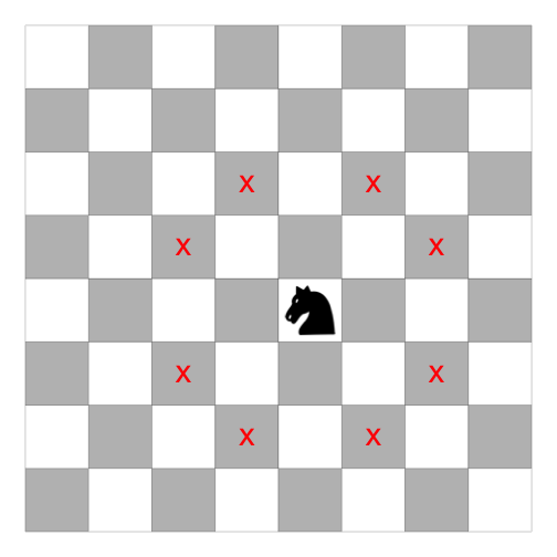
The first question is how we can simulate a knight’s move randomly. There are eight positions that a knight can move to, following the rule of “two spaces in one direction, one in the other”.

It helps to break each possible move into its X and Y components:
- X = 2, Y = 1
- X = 2, Y = -1
- X = 1, Y = 2
- X = 1, Y = -2
- X = -1, Y = 2
- X = -1, Y = -2
- X = -2, Y = 1
- X = -2, Y = -1
Notice that the moves are always made up of one 2 and one 1, and that either, both, or neither can be negative.
The first step of the simulation (getting a 1 and a 2) can be done as follows for a single simulation:
# Random number between 1 and 2
move_x <- sample(2, 1)

# If x is 2, y is 1, and vice versa
move_y <- 3 - move_x

c(move_x, move_y)
## [1] 1 2How about letting either number be negative? Well, sample(c(1, -1)) can get us a value that’s either 1 or -1, so we can multiply that by each.
move_x <- sample(2, 1) * sample(c(1, -1), 1)
move_y <- (3 - abs(move_x)) * sample(c(1, -1), 1)

c(move_x, move_y)
## [1] 2 -1Now that we can sample a single move, we can try sampling many moves (say, 20) by adding 20, replace = TRUE to each.
move_x <- sample(2, 20, replace = TRUE) * sample(c(1, -1), 20, replace = TRUE)
move_y <- (3 - abs(move_x)) * sample(c(1, -1), 20, replace = TRUE)

move_x
## [1] 2 1 1 1 -2 2 -2 1 2 -2 -1 1 -2 -2 2 -2 1 -2 -2 -2move_y## [1] 1 -2 -2 -2 1 1 1 -2 -1 -1 2 -2 -1 -1 -1 -1 -2 -1 1 -1Now that we’ve figured out how to simulate chess moves, we can go ahead with our simulation of positions.
Tidy simulation
The crossing() function from tidyr is wonderful for setting up Monte Carlo simulations. It creates a tbl_df with every combination of the inputs (it’s similar to the built-in expand.grid).
In this simulation we’ll want some number of trials and some number of turns. If we wanted to generate 3 trials that each included 3 chess turns, we could do:
crossing(trial = 1:3,
         turn = 1:3)
## # A tibble: 9 x 2
## trial turn
## <int> <int>
## 1 1 1
## 2 1 2
## 3 1 3
## 4 2 1
## 5 2 2
## 6 2 3
## 7 3 1
## 8 3 2
## 9 3 3In this experiment, we’ll simulate 100,000 trials (and, as the riddle specifies, 20 moves), and then bring in our vectorized approach to simulating chess moves. Notice we use n() (a special dplyr function) for the number of items.
# Use n() and replace = TRUE to vectorize the sampling above
crossing(trial = 1:100000,
         turn = 1:20) %>%
  mutate(move_x = sample(2, n(), replace = TRUE) *
           sample(c(1, -1), n(), replace = TRUE),
         move_y = (3 - abs(move_x)) *
           sample(c(1, -1), n(), replace = TRUE))
## # A tibble: 2,000,000 x 4
## trial turn move_x move_y
## <int> <int> <dbl> <dbl>
## 1 1 1 1 -2
## 2 1 2 2 -1
## 3 1 3 1 -2
## 4 1 4 -1 -2
## 5 1 5 -2 -1
## 6 1 6 -1 -2
## 7 1 7 1 -2
## 8 1 8 -2 1
## 9 1 9 1 -2
## 10 1 10 2 -1
## # ... with 1,999,990 more rowsNow, because the knights both start at (0, 0), we can calculate the position based on the cumulative sum of moves the X direction and in the Y direction. We do this by adding a group_by() (since movement happens separately within each trial) and mutate() to the sequence.
turns <- crossing(trial = 1:100000,
                  turn = 1:20) %>%
  mutate(move_x = sample(2, n(), replace = TRUE) *
           sample(c(1, -1), n(), replace = TRUE),
         move_y = (3 - abs(move_x)) *
           sample(c(1, -1), n(), replace = TRUE)) %>%
  group_by(trial) %>%
  mutate(position_x = cumsum(move_x),
         position_y = cumsum(move_y)) %>%
  ungroup()

turns
## # A tibble: 2,000,000 x 6
## trial turn move_x move_y position_x position_y
## <int> <int> <dbl> <dbl> <dbl> <dbl>
## 1 1 1 1 2 1 2
## 2 1 2 2 1 3 3
## 3 1 3 1 2 4 5
## 4 1 4 -2 -1 2 4
## 5 1 5 -1 2 1 6
## 6 1 6 2 -1 3 5
## 7 1 7 1 -2 4 3
## 8 1 8 2 1 6 4
## 9 1 9 2 -1 8 3
## 10 1 10 1 -2 9 1
## # ... with 1,999,990 more rowsJust like that, we’ve performed 100,000 trials of 20 sequential chess moves. Not bad!
Answering the questions
First, let’s answer the riddle’s question. How often is the knight back at its home space (0, 0) by the twentieth move?
turns %>%
  filter(turn == 20) %>%
  summarize(mean(position_x == 0 & position_y == 0))
## # A tibble: 1 x 1
## `mean(position_x == 0 & position_y == 0)`
## <dbl>
## 1 0.00627The probability of being back on the home space is about .6%.
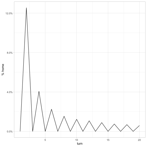
How does this compare to other turns?
library(ggplot2)
theme_set(theme_light())

by_turn <- turns %>%
  group_by(turn) %>%
  summarize(home = mean(position_x == 0 & position_y == 0))

by_turn %>%
  ggplot(aes(turn, home)) +
  geom_line() +
  scale_y_continuous(labels = scales::percent_format()) +
  labs(y = "% home")
It looks like it’s impossible for the knight to be back home on an odd numbered turn (if you have a chessboard you can try it!). At an even numbered turn, the probability is 1/8 for the second turn (the probability the first move was immediately followed by the opposite move). It then goes down from there to the .006 we see above.
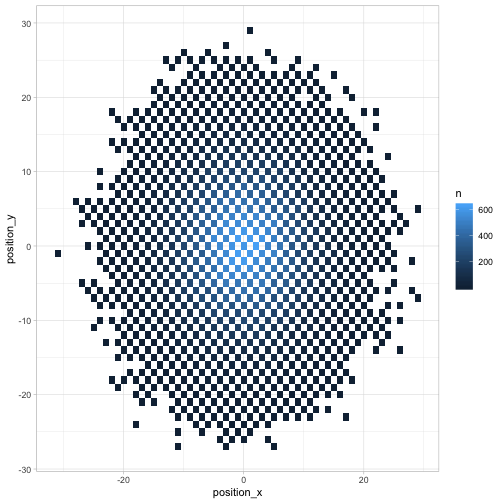
Where might the chess piece be by turn 20? A geom_tile is a nice visualization for this.
turns %>%
  filter(turn == 20) %>%
  count(position_x, position_y, sort = TRUE) %>%
  ggplot(aes(position_x, position_y, fill = n)) +
  geom_tile()
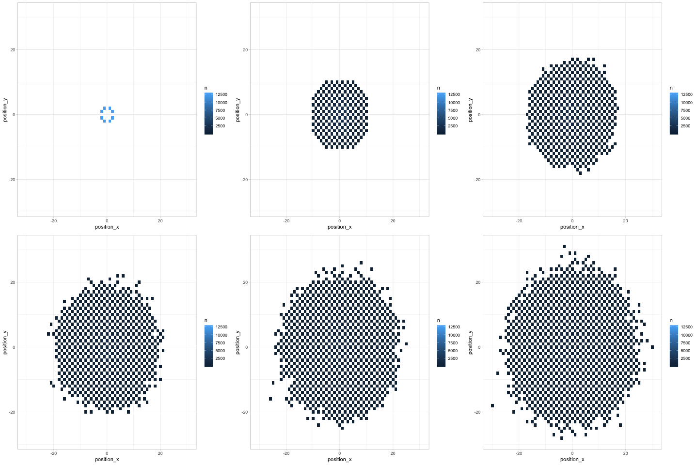
Finally, any time we look at change over time (especially in several dimensions like a chess board), we can use Thomas Pedersen’s gganimate package to give a more dynamic view.
library(gganimate)

turns %>%
  count(turn, position_x, position_y) %>%
  ggplot(aes(position_x, position_y, fill = n)) +
  geom_tile() +
  transition_manual(turn)
Besides showing how the knight “spreads” across the board, the animation communicates an insight that might not be noticeable otherwise (but which is relevant in chess): any given space on the chessboard is either an “odd # of moves” space or an “even # of moves” one. As we saw earlier, the home is an even space, so it can be reached on turn 20 but not on turns 19 or 21.
Conclusions
What have we learned about efficient simulation in R?
- Think vectorizably: Notice that we generated all of our 2 million moves in a couple of calls to
sample(). This helps keeps our simulation fast because functions likesample()have some computational overhead. If we’d simulated each individual move in a loop, this simulation would have taken a lot longer. - Some functions show up a lot in simulations. The
crossing()andcumsum()functions are very different, but they’re both wildly useful for simulations. Make sure you learn and understand them! - Tidy simulation is useful for visualization This puzzle could have been solved a bit more computationally efficiently by creating matrices for
move_x,move_y,position_x, andposition_y, and operating on them instead. In my opinion it would have made the code a bit less readable. But more importantly, by working in a tidy format we were able to immediately pipe the results into ggplot2 and gganimate and create visualizations. These helped check our results and improve our intuition around the answer.
Until next time, happy simulating!
