Understanding mixture models and expectation-maximization (using baseball statistics)

Previously in this series:

• Understanding the beta distribution
• Understanding empirical Bayes estimation
• Understanding credible intervals
• Understanding the Bayesian approach to false discovery rates
• Understanding Bayesian A/B testing
• Understanding beta binomial regression
• Understanding empirical Bayesian hierarchical modeling

In this series on empirical Bayesian methods on baseball data, we’ve been treating our overall distribution of batting averages as a beta distribution, which is a simple distribution between 0 and 1 that has a single peak. But what if that weren’t a good fit? For example, what if we had a multimodal distribution, with multiple peaks?

In this post, we’re going to consider what to do when your binomial proportions are made up of multiple peaks, and when you don’t know which observation belongs to which clusters. For example, so far in our analysis we’ve been filtering out pitchers, who tend to have a much lower batting average than non-pitchers. If you include them, the data looks something like this:

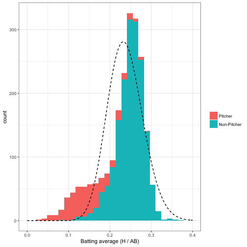
These batting averages certainly don’t look like a single beta distribution- it’s more like two separate ones mixed together. Imagine that you didn’t know which players were pitchers, and you wanted to separate the data into two groups according to your best prediction. This is very common in practical machine learning applications, such as clustering and segmentation.

In this post we’ll examine mixture models, where we treat the distribution of batting averages as a mixture of two beta-binomial distributions, and need to guess which player belongs to which group. This will also introduce the concept of an expectation-maximization algorithm, which is important in both Bayesian and frequentist statistics. We’ll show how to calculate a posterior probability for the cluster each player belongs to, and see that mixture models are still a good fit for the empirical Bayes framework.

Setup

As usual, I’ll start with some code you can use to catch up if you want to follow along in R. If you want to understand what it does in more depth, check out the previous posts in this series. (As always, all the code in this post can be found here).¹

library(dplyr)
library(tidyr)
library(Lahman)
library(ggplot2)
theme_set(theme_bw())

# Identify those who have pitched at least three games
pitchers <- Pitching %>%
  group_by(playerID) %>%
  summarize(gamesPitched = sum(G)) %>%
  filter(gamesPitched > 3)

# in this setup, we're keeping some extra information for later in the post:
# a "bats" column and a "year" column
career <- Batting %>%
  filter(AB > 0, lgID == "NL", yearID >= 1980) %>%
  group_by(playerID) %>%
  summarize(H = sum(H), AB = sum(AB), year = mean(yearID)) %>%
  mutate(average = H / AB,
         isPitcher = playerID %in% pitchers$playerID)

# Add player names
career <- Master %>%
  tbl_df() %>%
  dplyr::select(playerID, nameFirst, nameLast, bats) %>%
  unite(name, nameFirst, nameLast, sep = " ") %>%
  inner_join(career, by = "playerID")

We’ve been filtering out pitchers in the previous posts, which make batting averages look roughly like a beta distribution. But when we leave them in, as I showed above, the data looks a lot less like a beta:

The dashed density curve represents the beta distribution we would naively fit to this data. We can see that unlike our earlier analysis, where we’d filtered out pitchers, the beta is not a good fit- but that it’s plausible that we could fit the data using two beta distributions, one for pitchers and one for non-pitchers.

In this example, we know which players are pitchers and which aren’t. But if we didn’t, we would need to assign each player to a distribution, or “cluster”, before performing shrinkage on it. In a real analysis it’s not realistic that we wouldn’t know which players are pitchers, but it’s an excellent illustrative example of a mixture model and of expectation-maximization algorithms.

Expectation-maximization

The challenge of mixture models is that at the start, we don’t know which observations belong to which cluster, nor what the parameters of each distribution is. It’s difficult to solve these problems at the same time- so an expectation-maximization (EM) algorithm takes the jump of estimating them one at a time, and alternating between them.

The first thing to do in an EM clustering algorithm is to assign our clusters randomly:

set.seed(2016)

# We'll fit the clusters only with players that have had at least 20 at-bats
starting_data <- career %>%
  filter(AB >= 20) %>%
  select(-year, -bats, -isPitcher) %>%
  mutate(cluster = factor(sample(c("A", "B"), n(), replace = TRUE)))

Maximization

Now that we’ve got cluster assignments, what do the densities of each cluster look like?

starting_data %>%
  ggplot(aes(average, color = cluster)) +
  geom_density()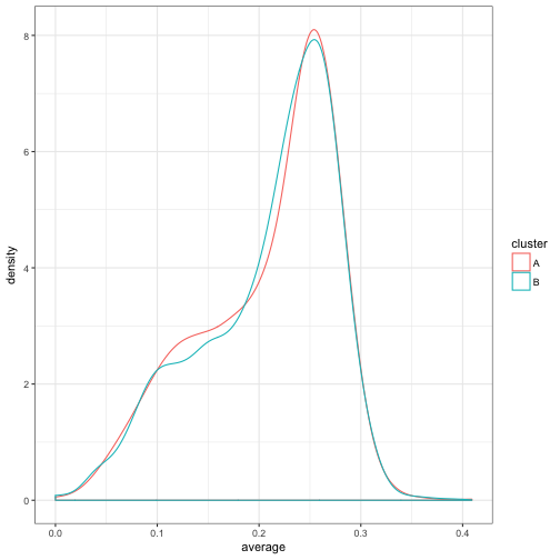

Well, that doesn’t look like much of a division- they have basically the same density! That’s OK: one of the nice features of expectation-maximization is that we don’t actually have to start with good clusters to end up with a good result.

We’ll now write a function for fitting a beta-binomial distribution using maximum likelihood estimation (and the dbetabinom.ab function from the VGAM package). This is a process we’ve done in multiple posts before, including the appendix of one of the first ones. We’re just encapsulating it into a function.

library(VGAM)

fit_bb_mle <- function(x, n) {
  # dbetabinom.ab is the likelihood function for a beta-binomial
  # using n, alpha and beta as parameters
  ll <- function(alpha, beta) {
    -sum(dbetabinom.ab(x, n, alpha, beta, log = TRUE))
  }
  m <- stats4::mle(ll, start = list(alpha = 3, beta = 10), method = "L-BFGS-B",
                   lower = c(0.001, .001))
  ab <- stats4::coef(m)
  data_frame(alpha = ab[1], beta = ab[2], number = length(x))
}

(The number column I added will be useful in the next step). For example, here are the alpha and beta chosen for the entire data as a whole:

fit_bb_mle(starting_data$H, starting_data$AB)

## # A tibble: 1 × 3
##   alpha  beta number
##   <dbl> <dbl>  <int>
## 1  12.8  45.5   3209

But now we’re working with a mixture model. This time, we’re going to fit the model within each of our (randomly assigned) clusters:

fits <- starting_data %>%
  group_by(cluster) %>%
  do(fit_bb_mle(.$H, .$AB)) %>%
  ungroup()

fits

## # A tibble: 2 × 4
##   cluster alpha  beta number
##    <fctr> <dbl> <dbl>  <int>
## 1       A  12.1  43.3   1559
## 2       B  13.6  47.9   1650

Another component of this model is the prior probability that a player is in cluster A or cluster B, which we set to 50-50 when we were assigning random clusters. We can estimate our new iteration of this based on the total number of assignments in each group, which is why we included the number column:

fits <- fits %>%
  mutate(prior = number / sum(number))

fits

## # A tibble: 2 × 5
##   cluster alpha  beta number prior
##    <fctr> <dbl> <dbl>  <int> <dbl>
## 1       A  12.1  43.3   1559 0.486
## 2       B  13.6  47.9   1650 0.514

Much as the within-cluster densities only changed a little, the priors only changed a little as well. This was the maximization step: find the maximum likelihood parameters (in this case, two alpha/beta values, and a per-cluster probability), pretending we knew the assignments.

Expectation

We now have a distribution for each cluster. It’s worth noting that these are pretty similar distributions, and that neither is a good fit to the data.

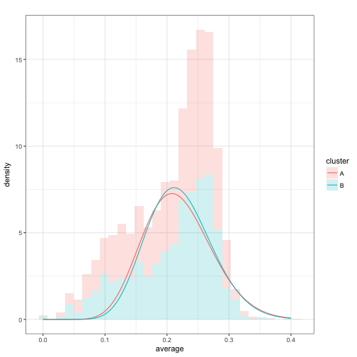
However, notice that due to a small random difference, cluster B is slightly more likely than cluster A for batting averages above about .2, and vice versa below .2.

Consider therefore that each player has a likelihood it would have been generated from cluster A, and a likelihood it would have been generated from cluster B (being sure to weight each by the prior probability of being in A or B):

crosses <- starting_data %>%
  select(-cluster) %>%
  crossing(fits) %>%
  mutate(likelihood = prior * VGAM::dbetabinom.ab(H, AB, alpha, beta))

crosses

## # A tibble: 6,418 × 11
##     playerID               name     H    AB average cluster alpha  beta
##        <chr>              <chr> <int> <int>   <dbl>  <fctr> <dbl> <dbl>
## 1  abbotje01        Jeff Abbott    11    42  0.2619       A  12.1  43.3
## 2  abbotje01        Jeff Abbott    11    42  0.2619       B  13.6  47.9
## 3  abbotji01         Jim Abbott     2    21  0.0952       A  12.1  43.3
## 4  abbotji01         Jim Abbott     2    21  0.0952       B  13.6  47.9
## 5  abbotku01        Kurt Abbott   475  1860  0.2554       A  12.1  43.3
## 6  abbotku01        Kurt Abbott   475  1860  0.2554       B  13.6  47.9
## 7  abbotky01        Kyle Abbott     3    31  0.0968       A  12.1  43.3
## 8  abbotky01        Kyle Abbott     3    31  0.0968       B  13.6  47.9
## 9  abercre01 Reggie Abercrombie    86   386  0.2228       A  12.1  43.3
## 10 abercre01 Reggie Abercrombie    86   386  0.2228       B  13.6  47.9
## # ... with 6,408 more rows, and 3 more variables: number <int>,
## #   prior <dbl>, likelihood <dbl>

For example, consider Jeff Abbott, who got 11 hits out of 42 at-bats. He had a 4.35% chance of getting that if he were in cluster A, but a 4.76% chance if he were in cluster B. For that reason (even though it’s a small difference), we’ll put him in B. Similarly we’ll put Kyle Abbott in cluster A: 3/31 was more likely to come from that distribution.

We can do that for every player using group_by and top_n:

assignments <- starting_data %>%
  select(-cluster) %>%
  crossing(fits) %>%
  mutate(likelihood = prior * VGAM::dbetabinom.ab(H, AB, alpha, beta)) %>%
  group_by(playerID) %>%
  top_n(1, likelihood) %>%
  ungroup()

assignments

## # A tibble: 3,209 × 11
##     playerID               name     H    AB average cluster alpha  beta
##        <chr>              <chr> <int> <int>   <dbl>  <fctr> <dbl> <dbl>
## 1  abbotje01        Jeff Abbott    11    42  0.2619       B  13.6  47.9
## 2  abbotji01         Jim Abbott     2    21  0.0952       B  13.6  47.9
## 3  abbotku01        Kurt Abbott   475  1860  0.2554       B  13.6  47.9
## 4  abbotky01        Kyle Abbott     3    31  0.0968       A  12.1  43.3
## 5  abercre01 Reggie Abercrombie    86   386  0.2228       B  13.6  47.9
## 6  abnersh01        Shawn Abner   110   531  0.2072       B  13.6  47.9
## 7  abreubo01        Bobby Abreu  1607  5395  0.2979       B  13.6  47.9
## 8  abreuto01         Tony Abreu   129   509  0.2534       B  13.6  47.9
## 9  acevejo01       Jose Acevedo     8   101  0.0792       A  12.1  43.3
## 10 aceveju01       Juan Acevedo     6    65  0.0923       A  12.1  43.3
## # ... with 3,199 more rows, and 3 more variables: number <int>,
## #   prior <dbl>, likelihood <dbl>

That’s the expectation step: assigning each person to the most likely cluster. How do our assignments look after that?

ggplot(assignments, aes(average, fill = cluster)) +
  geom_histogram()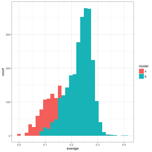

Something really important happened here: even though the two beta models we’d fit were very similar, we still split up the data rather neatly. Generally batters with a higher average ended up in cluster B, while batters with a lower average were in cluster A. (Note that due to B having a slightly higher prior probability, it was possible for players with a low average- but also a low AB- to be assigned to cluster B).

Expectation-Maximization

The above two steps got to a better set of assignments than our original, random ones. But there’s no reason to believe these are as good as we can get. So we repeat the two steps, choosing new parameters for each distribution in the mixture and then making new assignments each time.

For example, now that we’ve reassigned each player’s cluster, we could re-fit the beta-binomial with the new assignments. Those distributions would look like this:

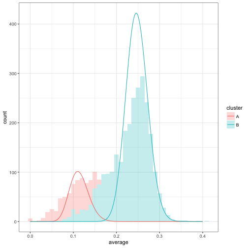
Unlike our first model fit, we can see that cluster A and cluster B have diverged a lot. Now we can take those parameters and perform a new estimation step. Generally we will do this multiple times, as an iterative process. This is the heart of an expectation-maximization algorithm, where we switch between assigning clusters (expectation) and fitting the model from those clusters (maximization).

set.seed(1337)

iterate_em <- function(state, ...) {
  fits <- state$assignments %>%
    group_by(cluster) %>%
    do(mutate(fit_bb_mle(.$H, .$AB), number = nrow(.))) %>%
    ungroup() %>%
    mutate(prior = number / sum(number))

  assignments <- assignments %>%
    select(playerID:average) %>%
    crossing(fits) %>%
    mutate(likelihood = prior * VGAM::dbetabinom.ab(H, AB, alpha, beta)) %>%
    group_by(playerID) %>%
    top_n(1, likelihood) %>%
    ungroup()
  
  list(assignments = assignments,
       fits = fits)
}

library(purrr)

iterations <- accumulate(1:5, iterate_em, .init = list(assignments = starting_data))

Here I used the accumulate function from the purrr package, which is useful for running data through the same function repeatedly and keeping intermediate states. I haven’t seen others use this tidy approach to EM algorithms, and there are existing R approaches to mixture models.² But I like this approach both because it’s transparent about what we’re doing in each iteration, and because our iterations are now combined in a tidy format, which is convenient to summarize and visualize.

For example, how did our assignments change over the course of the iteration?

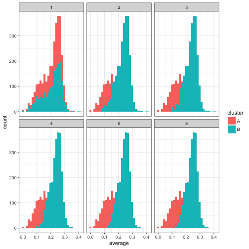
We notice that only the first few iterations led to a shift in the assignments, after which it appears to converge. Similarly, how did the estimated beta distributions change over these iterations?

fit_iterations <- iterations %>%
  map_df("fits", .id = "iteration")

fit_iterations %>%
  crossing(x = seq(.001, .4, .001)) %>%
  mutate(density = prior * dbeta(x, alpha, beta)) %>%
  ggplot(aes(x, density, color = iteration, group = iteration)) +
  geom_line() +
  facet_wrap(~ cluster)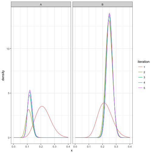

This confirms that it took about three iterations to converge, and then stayed about the same after that. Also notice that in the process, cluster B got much more likely than cluster A, which makes sense since there are more non-pitchers than pitchers in the dataset.

Assigning players to clusters

We now have some final parameters for each cluster:

## # A tibble: 2 × 6
##   iteration cluster alpha  beta number prior
##       <chr>  <fctr> <dbl> <dbl>  <int> <dbl>
## 1         5       A  43.0   312    740 0.231
## 2         5       B  98.3   292   2469 0.769

How would we assign players to clusters, and get a posterior probability that the player belongs to that cluster? Well, let’s arbitrarily pick the six players that each batted exactly 100 times:

batter_100 <- career %>%
  filter(AB == 100) %>%
  arrange(average)

batter_100

## # A tibble: 6 × 8
##    playerID            name   bats     H    AB  year average isPitcher
##       <chr>           <chr> <fctr> <int> <int> <dbl>   <dbl>     <lgl>
## 1 dejesjo01   Jose de Jesus      R    11   100  1990    0.11      TRUE
## 2 nicasju01    Juan Nicasio      R    12   100  2012    0.12      TRUE
## 3 mahonmi02    Mike Mahoney      R    18   100  2002    0.18     FALSE
## 4 cancero01 Robinson Cancel      R    20   100  2007    0.20     FALSE
## 5 buschmi01      Mike Busch      R    22   100  1996    0.22     FALSE
## 6 shealry01     Ryan Shealy      R    32   100  2006    0.32     FALSE

Where would we classify each of them? Well, we’d consider the likelihood each would get the number of hits they did if they were a pitcher (cluster A) or a non-pitcher (cluster B):

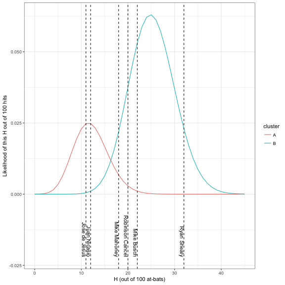
By Bayes’ Theorem, we can simply use the ratio of one likelihood (say, A in red) to the sum of the two likelihoods to get the posterior probability:

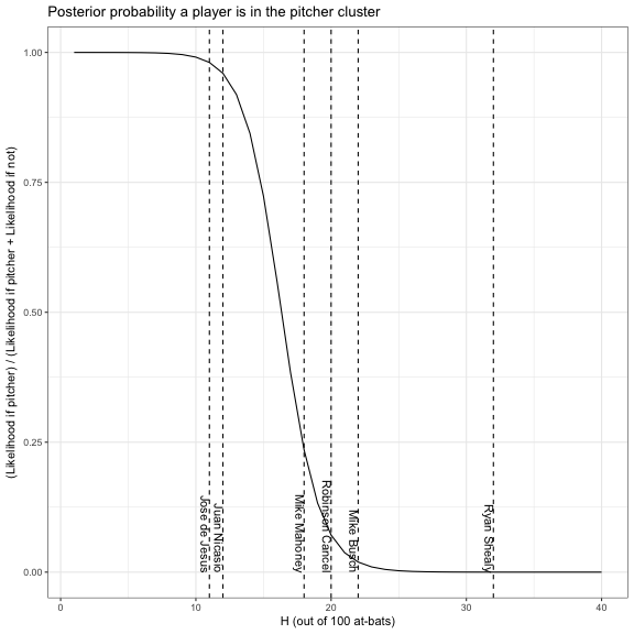
Based on this, we feel confident that Juan Nicasio and Jose de Jesus are pitchers, and that the others probably aren’t. And we’d be right! (Check out the isPitcher column in the batter_100 table above).

This allows us to assign all players in the dataset to one of the two clusters.

career_likelihoods <- career %>%
  filter(AB > 20) %>%
  crossing(final_parameters) %>%
  mutate(likelihood = prior * VGAM::dbetabinom.ab(H, AB, alpha, beta)) %>%
  group_by(playerID) %>%
  mutate(posterior = likelihood / sum(likelihood))

career_assignments <- career_likelihoods %>%
  top_n(1, posterior) %>%
  ungroup()

Since we know whether each player actually is a pitcher or not, we can also get a confusion matrix. How many pitchers were accidentally assigned to cluster B, and how many non-pitchers were assigned to cluster A? In this case we’ll look only at the ones for which we had at least 80% confidence in our classification.

career_assignments %>%
  filter(posterior > .8) %>%
  count(isPitcher, cluster) %>%
  spread(cluster, n)

## Source: local data frame [2 x 3]
## Groups: isPitcher [2]
## 
##   isPitcher     A     B
## *     <lgl> <int> <int>
## 1     FALSE    23  2026
## 2      TRUE   493   157

Not bad, considering the only information we used was the batting average- and note that we didn’t even use data on who were pitchers to train the model, but just let the clusters define themselves.

It looks like we were a lot more likely to call a pitcher a non-pitcher than vice versa. There’s a lot more we could do to examine this model, how well calibrated its posterior estimates are, and what kinds of pitchers may be mistaken for non-pitchers (e.g. good batters who pitched only a few times), but we won’t consider them in this post.

Empirical bayes shrinkage with a mixture model

We’ve gone to all this work posterior probabilities of each player’s assignments. How can we use this in empirical Bayes shrinkage, or with the other methods we’ve described in this series?

Well, consider that all of our other methods have worked because the posterior was another beta distribution (thanks to the beta being the conjugate prior of the binomial). However, now that each point might belong to one of two beta distributions, our posterior will be a mixture of betas. This mixture is made up of the posterior from each cluster, weighted by the probability the point belongs to that cluster.

For example, consider the six players who had exactly 100 at-bats. Their posterior distributions would look like this:

batting_data <- career_likelihoods %>%
  ungroup() %>%
  filter(AB == 100) %>%
  mutate(name = paste0(name, " (", H, "/", AB, ")"),
         name = reorder(name, H),
         alpha1 = H + alpha,
         beta1 = AB - H + beta)

batting_data %>%
  crossing(x = seq(0, .4, .001)) %>%
  mutate(posterior_density = posterior * dbeta(x, alpha1, beta1)) %>%
  group_by(name, x) %>%
  summarize(posterior_density = sum(posterior_density)) %>%
  ggplot(aes(x, posterior_density, color = name)) +
  geom_line(show.legend = FALSE) +
  geom_vline(aes(xintercept = average), data = batting_data, lty = 2) +
  facet_wrap(~ name) +
  labs(x = "Batting average (actual average shown as dashed line)",
       y = "Posterior density after updating")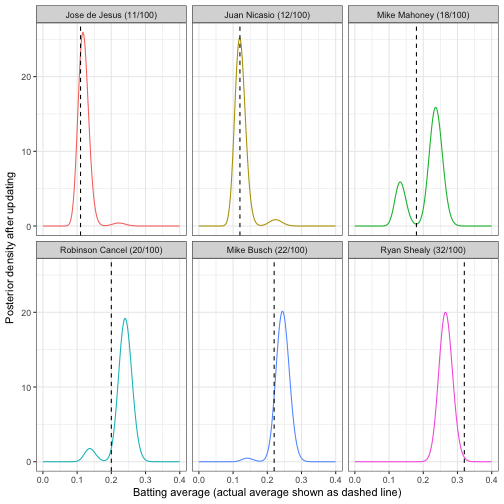

For example, we are pretty sure that Jose de Jesus and Juan Nicasio are part of the “pitcher” cluster, so that makes up most of their posterior mass, and all of Ryan Shealy’s density is in the “non-pitcher” cluster. However, we’re pretty split on Mike Mahoney- he could be a pitcher who is unusually good at batting, or a non-pitcher who is unusually bad.

Can we perform shrinkage like we did in that early post? If our goal is still to find the mean of each posterior, then yes! Thanks to linearity of expected value, we can simply average the two distribution means, weighing each by the probability the player belongs to that cluster:

eb_shrinkage <- career_likelihoods %>%
  mutate(shrunken_average = (H + alpha) / (AB + alpha + beta)) %>%
  group_by(playerID) %>%
  summarize(shrunken_average = sum(posterior * shrunken_average))

For example, we are pretty sure that Jose de Jesus and Juan Nicasio are part of the “pitcher” cluster, which means they mostly get shrunken towards that center. We are quite certain Ryan Shealy is not a pitcher, so he’ll be updated based entirely on that distribution.

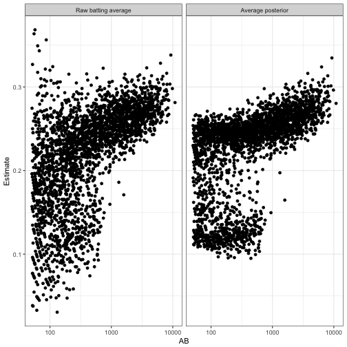
Notice that instead of shrinking towards a single value, the batting averages are now shrunken towards two centers: one higher value for the non-pitcher cluster, one smaller value for the pitcher cluster. Ones that are exactly in between don’t really get shrunken in either direction- they’re “pulled equally”.

(For simplicity’s sake I didn’t use our beta-binomial regression approach in this model, but that could easily be added to take into account the relationship between average and AB).

Not all of the methods we’ve used in this series are so easy to adapt to a multimodal distribution. For example, a credible interval is ambiguous in a multimodal distribution (see here for more), and we’d need to rethink our approach to Bayesian A/B testing. But since we do have a posterior distribution for each player- even though it’s not a beta- we’d be able to face these challenges.

What’s Next: Combining into an R package

We’ve introduced a number of statistical techniques in this series for dealing with empirical Bayes, the beta-binomial relationship, A/B testing, etc. Since I’ve provided the code at each stage, you could certainly apply these methods to your own data (as some already have!). However, you’d probably find yourself copying and pasting a rather large amount of code, which isn’t necessarily something you want to do every time you run into this kind of binomial data (it takes you out of the flow of your own data analysis).

In my next post I’ll introduce an R package for performing empirical Bayes on binomial data that encapsulates many of the analyses we’ve performed in this series. These statistical techniques aren’t original to me (most can be found in an elementary Bayesian statistics textbook), but providing them in a convenient R package can still be useful for the community. We’ll also go over some of the choices one makes in developing a statistics package in R, particularly one that is compatible with the tidy tools we’ve been using.