The 'largest stock profit or loss' puzzle: efficient computation in R

Previously in this series:

• The “lost boarding pass” puzzle
• The “deadly board game” puzzle
• The “knight on an infinite chessboard” puzzle

I recently came across an interview problem from A Cool SQL Problem: Avoiding For-Loops . Avoiding loops is a topic I always enjoy reading about, and the blog post didn’t disappoint. I’ll quote that post’s description of the problem:

You have a table of trading days (with no gaps) and close prices for a stock.

Find the highest and lowest profits (or losses) you could have made if you bought the stock at one close price and sold it at another close price, i.e. a total of exactly two transactions.

You cannot sell a stock before it has been purchased. Your solution can allow buying and selling on the same trading_date (i.e. profit or loss of $0 is always, by definition, an available option); however, for some bonus points, you may write a more general solution for this problem that requires you to hold the stock for at least N days.

The blog post provided a SQL solution, and noted the importance of thinking with tables rather than loops. But the post made me think about how I’d solve the problem in R, and make the solution as computationally efficient as possible. As in many of my posts, we’ll take a “tidy approach” that focuses on the dplyr, tidyr, and ggplot2 packages.

Setup: Getting stock data with the tidyquant package

The original blog post worked on just one stock symbol, but let’s make the problem slightly harder by examining data for several stocks at the same time. To gather some real data, I’ll use the excellent tidyquant package from Business Science. I’ll pick four stocks: Apple, Microsoft, Netflix, and Tesla.

library(tidyverse)
library(tidyquant)

stock_symbols <- c("AAPL", "MSFT", "NFLX", "TSLA")

# Keep just the closing price
stock_prices <- tq_get(stock_symbols, from = "2010-01-01") %>%
  select(symbol, date, close)

stock_prices

## # A tibble: 9,922 x 3
##    symbol date       close
##    <chr>  <date>     <dbl>
##  1 AAPL   2010-01-04  30.6
##  2 AAPL   2010-01-05  30.6
##  3 AAPL   2010-01-06  30.1
##  4 AAPL   2010-01-07  30.1
##  5 AAPL   2010-01-08  30.3
##  6 AAPL   2010-01-11  30.0
##  7 AAPL   2010-01-12  29.7
##  8 AAPL   2010-01-13  30.1
##  9 AAPL   2010-01-14  29.9
## 10 AAPL   2010-01-15  29.4
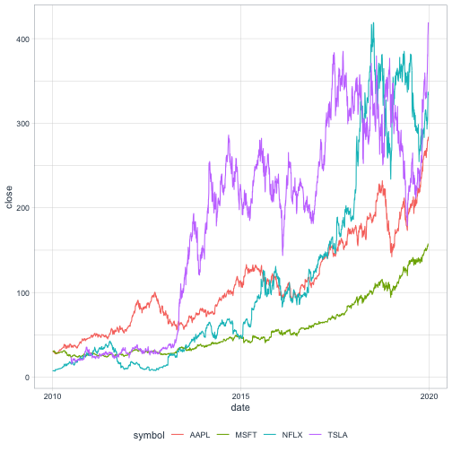
## # … with 9,932 more rows

Notice that the result from tq_get is tidy: one row per symbol per day. This isn’t part of the interview question, but we can visualize the stocks over time using ggplot2.

# In honor of the tidyquant package, we'll use theme_tq
theme_set(theme_tq())

ggplot(stock_prices, aes(date, close, color = symbol)) +
  geom_line() +
  theme_tq()

Solving the problem with a self-join

One way to approach this problem (one taken in SQL by the original blog post) is to cross join the data with itself, and examine all combinations of dates with a future date.

In this case, since we have the symbol column and we only want to compare symbols to themselves, we’ll want to join based on the "symbol" column.¹

library(tidyr)

stock_prices %>%
  inner_join(stock_prices,
             by = "symbol",
             suffix = c("", "_future"))

## # A tibble: 24,622,684 x 5
##    symbol date       close date_future close_future
##    <chr>  <date>     <dbl> <date>             <dbl>
##  1 AAPL   2010-01-04  30.6 2010-01-04          30.6
##  2 AAPL   2010-01-04  30.6 2010-01-05          30.6
##  3 AAPL   2010-01-04  30.6 2010-01-06          30.1
##  4 AAPL   2010-01-04  30.6 2010-01-07          30.1
##  5 AAPL   2010-01-04  30.6 2010-01-08          30.3
##  6 AAPL   2010-01-04  30.6 2010-01-11          30.0
##  7 AAPL   2010-01-04  30.6 2010-01-12          29.7
##  8 AAPL   2010-01-04  30.6 2010-01-13          30.1
##  9 AAPL   2010-01-04  30.6 2010-01-14          29.9
## 10 AAPL   2010-01-04  30.6 2010-01-15          29.4
## # … with 24,721,994 more rows

This creates all combinations of present and future dates, ending up in columns close and close_future. Now we’ll need a few dplyr steps:

• Filter for cases where date_future is greater than date (filter)
• Look at the change if you bought on date and sold on date_future (mutate)
• Aggregate to find the maximum and minimum change within each symbol (group_by/summarize)

So our solution looks like this:

stock_prices %>%
  inner_join(stock_prices,
             by = "symbol",
             suffix = c("", "_future")) %>%
  filter(date_future >= date) %>%
  mutate(change = close_future - close) %>%
  group_by(symbol) %>%
  summarize(largest_gain = max(change),
            largest_loss = min(change))

## # A tibble: 4 x 3
##   symbol largest_gain largest_loss
##   <chr>         <dbl>        <dbl>
## 1 AAPL           266.        -89.9
## 2 MSFT           136.        -21.5
## 3 NFLX           412.       -185. 
## 4 TSLA           415.       -206.

I don’t know if this metric is at all meaningful from a finance perspective (of course nobody would know in advance when you’re supposed to buy and sell a stock to maximize a stock), but it’s interesting to see how much Netflix has grown since 2010, and how Tesla has seen a large drop (though based on the graph above it has since recovered).

The above lines up with the original blog post: join the data to itself while constraining on comparing dates to future dates. However, in R, on a dataset this size, it’s not a very fast approach. It had to create a 25-million row table (~6.3 million for each symbol; the number of days squared), and it had to make millions of comparisons. On my machine it takes about 3 seconds to run, and if we’d had a dataset of thousands of symbols it would have been impossible.

Solving with vectorized functions: cummean and cummax

A much faster approach in R is to use vectorized functions. In particular, we can use cummax() (cumulative max) and cummin() (cumulative min), to quickly discover the highest and lowest future prices from each date.

We first sort by the stock symbol² and by the descending date. We also group by the symbol, which means we’ll be looking at changes within each stock.

stock_prices %>%
  arrange(symbol, desc(date)) %>%
  group_by(symbol) %>%
  mutate(highest_future = cummax(close),
         lowest_future = cummin(close))

## # A tibble: 9,922 x 5
## # Groups:   symbol [4]
##    symbol date       close highest_future lowest_future
##    <chr>  <date>     <dbl>          <dbl>         <dbl>
##  1 AAPL   2019-12-23  284             284          284 
##  2 AAPL   2019-12-20  279.            284          279.
##  3 AAPL   2019-12-19  280.            284          279.
##  4 AAPL   2019-12-18  280.            284          279.
##  5 AAPL   2019-12-17  280.            284          279.
##  6 AAPL   2019-12-16  280.            284          279.
##  7 AAPL   2019-12-13  275.            284          275.
##  8 AAPL   2019-12-12  271.            284          271.
##  9 AAPL   2019-12-11  271.            284          271.
## 10 AAPL   2019-12-10  268.            284          268.
## # … with 9,912 more rows

Look, for instance, at the 10th row of the table. The closing price of AAPL on 2019-12-10 was 268, and the highest it will ever be in the future is 284, while the lowest it will ever be is 268. This means that someone buying on 2019-12-10 could gain up to $16, and couldn’t lose money.

By finding the largest/smallest difference between each day’s price and the highest/lowest future price, we can get the highest possible gain or the biggest possible loss. This gives us a new approach to the interview problem.

stock_prices %>%
  arrange(symbol, desc(date)) %>%
  group_by(symbol) %>%
  summarize(highest_gain = max(cummax(close) - close),
            biggest_loss = min(cummin(close) - close))

## # A tibble: 4 x 3
##   symbol highest_gain biggest_loss
##   <chr>         <dbl>        <dbl>
## 1 AAPL           266.        -89.9
## 2 MSFT           136.        -21.5
## 3 NFLX           412.       -185. 
## 4 TSLA           415.       -206.

In R, this is about 1000X faster than the self-join approach (for me it takes about 5 milliseconds, compared to about 3 seconds for self-join). cummin and cummax are fast (they’re base R functions implemented in C), and the effect on memory is linear in terms of the number of observations.

It’s worth mentioning that the vectorized approach isn’t specific to dplyr (though dplyr makes it especially convenient for performing within each stock symbol). If x is an ordered vector, you can use rev(cummax(rev(x))) to get the highest future gain, which gives us a one liner for performing this on a vector of prices.

# Using the vector of prices from the ryx,r blog post
x <- c(41, 43, 47, 42, 45, 39,  38, 41)

max(rev(cummax(rev(x))) - x)

## [1] 6

min(rev(cummin(rev(x))) - x)

## [1] -9

Variation: waiting at least N days?

There’s one more variation from the original blog post that’s worth thinking through. What if you set the rule that you have to hold the stock for some number N (say, 100) of trading days N before selling it?

You can solve this in R with the dplyr’s lag() window function, which shifts each value in a vector several positions later.

# Separated into a mutate and a summarize just for the sake of clarity
stock_prices %>%
  arrange(symbol, desc(date)) %>%
  group_by(symbol) %>%
  mutate(highest_future = lag(cummax(close), 100),
         lowest_future = lag(cummin(close), 100)) %>%
  summarize(highest_gain = max(highest_future - close, na.rm = TRUE),
            biggest_loss = min(lowest_future - close, na.rm = TRUE))

## # A tibble: 4 x 3
##   symbol highest_gain biggest_loss
##   <chr>         <dbl>        <dbl>
## 1 AAPL           257.        -73.7
## 2 MSFT           134.        -16.7
## 3 NFLX           412.       -185. 
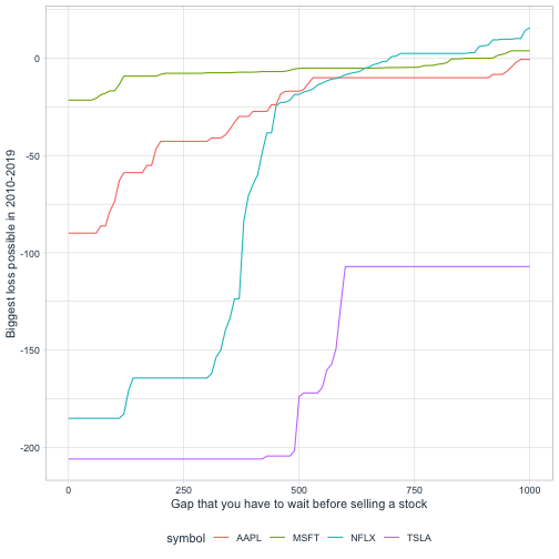
## 4 TSLA           403.       -206.

From this we can see that if we had to wait 100 days, our “highest possible gain” doesn’t change, but our “biggest possible loss” shrinks for some of them. This makes sense because these stocks have generally been growing over time.

What if we wanted to see how the N (the gap we have to wait) changes the biggest gain and biggest loss? Well, one of my favorite tidyr tricks is crossing(), which duplicates a dataset multiple times. By duplicating the data for many values of N, then doing lag(cummax(close), N[1]), we can calculate a solution for many values of N, and visualize them.

biggest_changes <- stock_prices %>%
  crossing(N = seq(0, 1000, 10)) %>%
  arrange(N, symbol, desc(date)) %>%
  group_by(N, symbol) %>%
  mutate(highest_future = lag(cummax(close), N[1]),
         lowest_future = lag(cummin(close), N[1])) %>%
  summarize(highest_gain = max(highest_future - close, na.rm = TRUE),
            biggest_loss = min(lowest_future - close, na.rm = TRUE))

biggest_changes %>%
  ggplot(aes(N, biggest_loss, color = symbol)) +
  geom_line() +
  labs(x = "Gap that you have to wait before selling a stock",
       y = "Biggest loss possible in 2010-2019")

This extension was made possible by two features of our approach:

• Advantage of the tidyverse: Since we solved the problem with dplyr, it was fairly straightforward to examine the effect of another parameter (N, the number of days we had to wait) by adding an extra group_by variable.
• Advantage of computational speed: Since we managed to solve the problem in milliseconds rather than seconds, it wasn’t much of a hassle to solve it for a hundred different input parameters.